07. Principal Component Analysis in R and SAS • TempleCBE

Author: Darina Chudnovskaya (darina.c@temple.edu)
Reviewers: J. Kyle Armstrong (tus75918@temple.edu, @jkylearmstrong-temple)
Affiliation: Lewis Katz School of Medicine at Temple University, Center for Biostatistics & Epidemiology

Introduction: Dimension Reduction in Clinical and Exploratory Data Analysis

Principal Component Analysis (PCA) is an unsupervised machine learning and exploratory data analysis (EDA) technique widely utilized across biostatistics, clinical trials, and epidemiological research. When analyzing large cohorts with extensive clinical measurements—such as repeated physiological scores, biomarker panels, and intensive care metrics—investigators often face high dimensionality and severe multicollinearity.

As summarized by biostatistician Darina Chudnovskaya:

“To put all this simply, just think of principal components as new axes that provide the best angle to see and evaluate the data, so that the differences between the observations are better visible.”

— Darina Chudnovskaya (citing builtin.com)

PCA reduces the dimensionality of multivariate continuous datasets by transforming correlated variables into a smaller set of uncorrelated, orthogonal variables known as Principal Components (PCs). Each principal component is a linear combination of the original variables, structured such that: 1. The first principal component ( $PC_1$ ) captures the maximum possible variance in the data. 2. Each subsequent component ( $PC_2, PC_3, \dots$ ) captures the maximum possible remaining variance under the mathematical constraint that it is orthogonal (uncorrelated) to all preceding components. 3. The total variance across all principal components equals the total variance of the original variables.

While principal components themselves are linear combinations and may not have a single physical unit of measurement, analyzing their loadings (eigenvectors) and eigenvalues reveals underlying data structures, detects clustering, and helps researchers select representative covariates for downstream multivariable survival modeling (such as cox_multi()).

The 5-Step PCA Mathematical Workflow

The mathematical execution of PCA proceeds through five fundamental steps:

  ┌─────────────────────────────────────────────────────────────┐
  │ 1. Standardize Continuous Variables (z-score scaling)       │
  └──────────────────────────────┬──────────────────────────────┘
                                 ▼
  ┌─────────────────────────────────────────────────────────────┐
  │ 2. Compute Covariance / Correlation Matrix (Σ or R)         │
  └──────────────────────────────┬──────────────────────────────┘
                                 ▼
  ┌─────────────────────────────────────────────────────────────┐
  │ 3. Compute Eigenvalues & Eigenvectors (Σ v = λ v)           │
  └──────────────────────────────┬──────────────────────────────┘
                                 ▼
  ┌─────────────────────────────────────────────────────────────┐
  │ 4. Retain Significant PCs (Kaiser Criterion & Scree Plot)   │
  └──────────────────────────────┬──────────────────────────────┘
                                 ▼
  ┌─────────────────────────────────────────────────────────────┐
  │ 5. Project Data onto Principal Axes (Feature Matrix X V)    │
  └─────────────────────────────────────────────────────────────┘

Standardize Variables: Because PCA is sensitive to measurement scales (variables with larger numerical ranges would spuriously dominate the variance), features are centered to mean zero ( $\mu = 0$ ) and scaled to unit variance ( $\sigma = 1$ ): $z_{ij} = \frac{x_{ij} - \bar{x}_j}{s_j}$ Standardizing is mathematically equivalent to performing PCA on the correlation matrix $\mathbf{R}$ rather than the unscaled covariance matrix $\mathbf{\Sigma}$ .
Calculate Correlation / Covariance Matrix: A symmetric $p \times p$ correlation matrix $\mathbf{R}$ is computed, capturing all pairwise linear relationships and correlation directions ( $+1$ to $-1$ ).
Calculate Eigenvalues and Eigenvectors: Eigen-decomposition solves the characteristic equation: $\det(\mathbf{R} - \lambda \mathbf{I}) = 0 \quad \implies \quad \mathbf{R} \mathbf{v}_k = \lambda_k \mathbf{v}_k$
- Eigenvalues ( $\lambda_k$ ): Represent the variance explained by the $k$ -th principal component. In standardized PCA with $p$ variables, $\sum_{k=1}^p \lambda_k = p$ .
- Eigenvectors ( $\mathbf{v}_k$ ): Unit-length directional vectors defining the principal axes (loadings).
Select Principal Components:
- Kaiser-Guttman Criterion: Retain components with eigenvalues $\lambda_k \ge 1$ (explaining more variance than an individual original standardized variable).
- Scree Plot Elbow: Identify the inflection point where additional components yield diminishing marginal variance.
- Cumulative Variance Threshold: Retain enough components to explain a pre-specified proportion of variance (typically 70%–80%).
Recast Observations onto Principal Component Axes: Observations are projected onto the retained eigenvectors to generate principal component scores: $\mathbf{Y} = \mathbf{Z} \mathbf{V}_k$

SAS and R Equivalence: The Iris Benchmark

To validate numerical equivalence between SAS PROC PRINCOMP and TempleCBE::run_pca(), we evaluate Fisher’s Iris dataset (150 observations across 4 morphometric variables: Sepal.Length, Sepal.Width, Petal.Length, Petal.Width).

SAS PROC PRINCOMP Implementation

In SAS, principal component analysis on standardized variables is invoked using PROC PRINCOMP:

/* SAS PROC PRINCOMP Benchmark */
proc princomp data=sashelp.iris out=iris_pca plots=all;
   var SepalLength SepalWidth PetalLength PetalWidth;
run;

TempleCBE run_pca Implementation

In R using TempleCBE, the equivalent workflow is executed via run_pca():

# Execute standardized PCA with TempleCBE
iris_pca <- run_pca(iris, scale = TRUE)
iris_pca
#> # A tibble: 4 × 6
#>   component eigenvalue difference proportion variance_pct cum_variance_pct
#>   <chr>          <dbl>      <dbl>      <dbl>        <dbl>            <dbl>
#> 1 PC1           2.92        2.00     0.730         73.0               73.0
#> 2 PC2           0.914       0.767    0.229         22.9               95.8
#> 3 PC3           0.147       0.126    0.0367         3.67              99.5
#> 4 PC4           0.0207     NA        0.00518        0.518            100

Numerical Concordance: SAS vs. TempleCBE

TempleCBE::run_pca() mirrors the exact output table produced by SAS PROC PRINCOMP. The listing SAS 9.4 produced for these 150 rows is committed (inst/sas/benchmark_princomp_iris.sas and inst/sas/list/benchmark_princomp_iris.lst), and the package tests compare run_pca() with it: eigenvalues and differences to the 8 decimals SAS prints, proportions to its 4.

Principal Component	Eigenvalue ( $\lambda$ )	Difference	Proportion of Variance	Cumulative Variance
PC1	2.9185	2.0045	72.96%	72.96%
PC2	0.9140	0.7673	22.85%	95.81%
PC3	0.1468	0.1261	3.67%	99.48%
PC4	0.0207	—	0.52%	100.00%

Notice that the first two principal components capture 95.81% of the total variance in the Iris dataset, allowing a 4-dimensional feature space to be represented in two dimensions with negligible loss of information.

Visualizing PCA: Scree Plots, Biplots, and Correlation Circles

TempleCBE provides comprehensive visualization functions adhering to institutional design standards.

1. Scree Plot with Kaiser-Guttman Threshold

The scree plot displays eigenvalues across components, highlighting the $\lambda = 1$ Kaiser criterion:

pca_scree_plot(iris_pca, metric = "eigenvalue", kaiser = TRUE)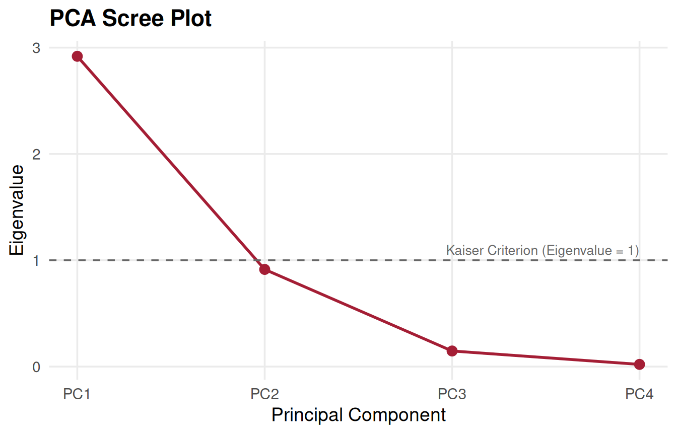

Scree plot with Kaiser criterion threshold.

Only $PC_1$ exceeds the Kaiser threshold ( $\lambda_1 = 2.92 > 1.0$ ), while $PC_2$ ( $\lambda_2 = 0.91$ ) is near the threshold and brings cumulative explained variance to 95.8%.

2. Variable Correlation Circle

The correlation circle illustrates how each original variable correlates with $PC_1$ and $PC_2$ on the unit circle:

pca_variables_plot(iris_pca, x = 1, y = 2)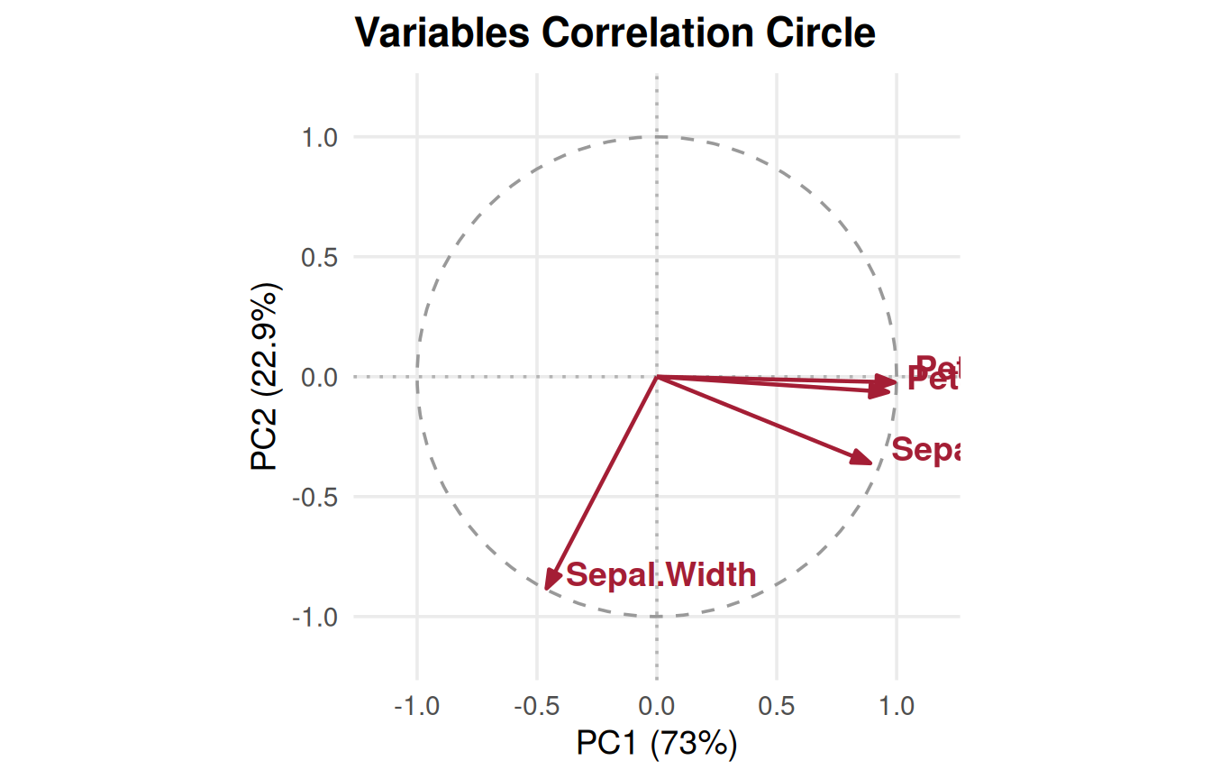

Variable correlation circle on the unit circle.

Interpretation: - Petal.Length, Petal.Width, and Sepal.Length exhibit strong positive correlations with $PC_1$ (vectors extending to the right). - Sepal.Width is nearly orthogonal to the petal dimensions and projects predominantly along $PC_2$ (vector extending upward).

3. Loadings Biplot with 95% Concentration Ellipses

The biplot projects individual observations along with variable loading vectors, with optional grouping and 95% confidence/concentration ellipses:

pca_biplot(iris_pca, group = iris$Species, ellipse = TRUE, percent = TRUE, title = "Iris PCA Biplot with 95% Concentration Ellipses")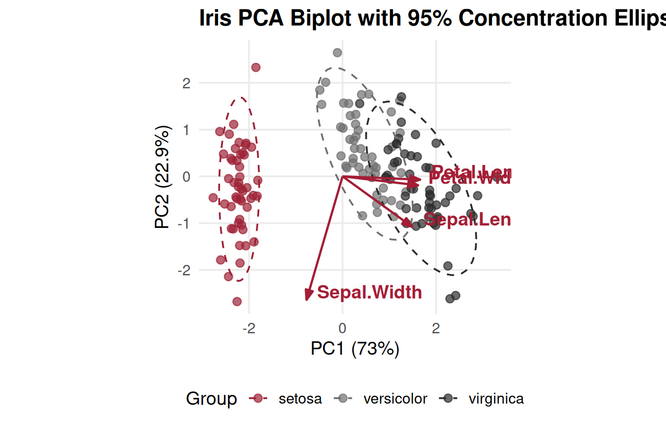

PCA biplot showing observation scores, variable vectors, and species clusters.

The biplot demonstrates complete separation of Iris setosa along $PC_1$ , driven by smaller petal dimensions and broader sepal width.

Clinical Application: Dimensionality Reduction for Survival Analysis

In clinical observational studies, researchers frequently collect multiple correlated physiological and procedural measurements. For example, consider an ICU cohort with 165 patients tracking: - Temperature Alteration Scores (TAS): tas_baseline, tas_min, tas_max, tas_ave - Demographics: age - Hospital Course: los_icu (ICU length of stay), los_hosp (hospital length of stay)

Simulating a Clinical Cohort

set.seed(42)
n <- 165

# Latent physiological severity and hospital course
severity <- rnorm(n, 0, 1)
exposure <- 0.6 * severity + rnorm(n, 0, 0.8)

clinical_data <- tibble(
  age = round(60 + 8 * severity + rnorm(n, 0, 5)),
  tas_baseline = round(37.5 + 0.8 * severity + rnorm(n, 0, 0.4), 1),
  tas_min = round(35.5 - 0.5 * severity + rnorm(n, 0, 0.3), 1),
  tas_max = round(38.8 + 1.1 * severity + rnorm(n, 0, 0.5), 1),
  tas_ave = round(37.2 + 0.7 * severity + rnorm(n, 0, 0.3), 1),
  los_icu = pmax(1, round(5 + 3 * exposure + rexp(n, 0.2))),
  los_hosp = pmax(2, round(12 + 5 * exposure + rexp(n, 0.1)))
)

head(clinical_data)
#> # A tibble: 6 × 7
#>     age tas_baseline tas_min tas_max tas_ave los_icu los_hosp
#>   <dbl>        <dbl>   <dbl>   <dbl>   <dbl>   <dbl>    <dbl>
#> 1    75         38.9    34.6    40.7    38.4      12       23
#> 2    53         37.4    36.2    37.7    36.6       5       36
#> 3    59         37.3    35.3    38.2    37.3       8       20
#> 4    66         38.1    35.4    39.5    38        16       15
#> 5    68         37.8    35.8    39.2    37.8      19       24
#> 6    59         37.8    35.6    38.7    37.3      11       53

Performing Clinical PCA

clin_pca <- run_pca(clinical_data, scale = TRUE)
clin_pca
#> # A tibble: 7 × 6
#>   component eigenvalue difference proportion variance_pct cum_variance_pct
#>   <chr>          <dbl>      <dbl>      <dbl>        <dbl>            <dbl>
#> 1 PC1            4.19      3.09       0.598         59.8              59.8
#> 2 PC2            1.09      0.251      0.156         15.6              75.4
#> 3 PC3            0.840     0.565      0.120         12.0              87.4
#> 4 PC4            0.274     0.0322     0.0392         3.92             91.3
#> 5 PC5            0.242     0.0421     0.0346         3.46             94.7
#> 6 PC6            0.200     0.0321     0.0286         2.86             97.6
#> 7 PC7            0.168    NA          0.0240         2.40            100

Clinical Scree Plot and Factor Interpretation

pca_scree_plot(clin_pca)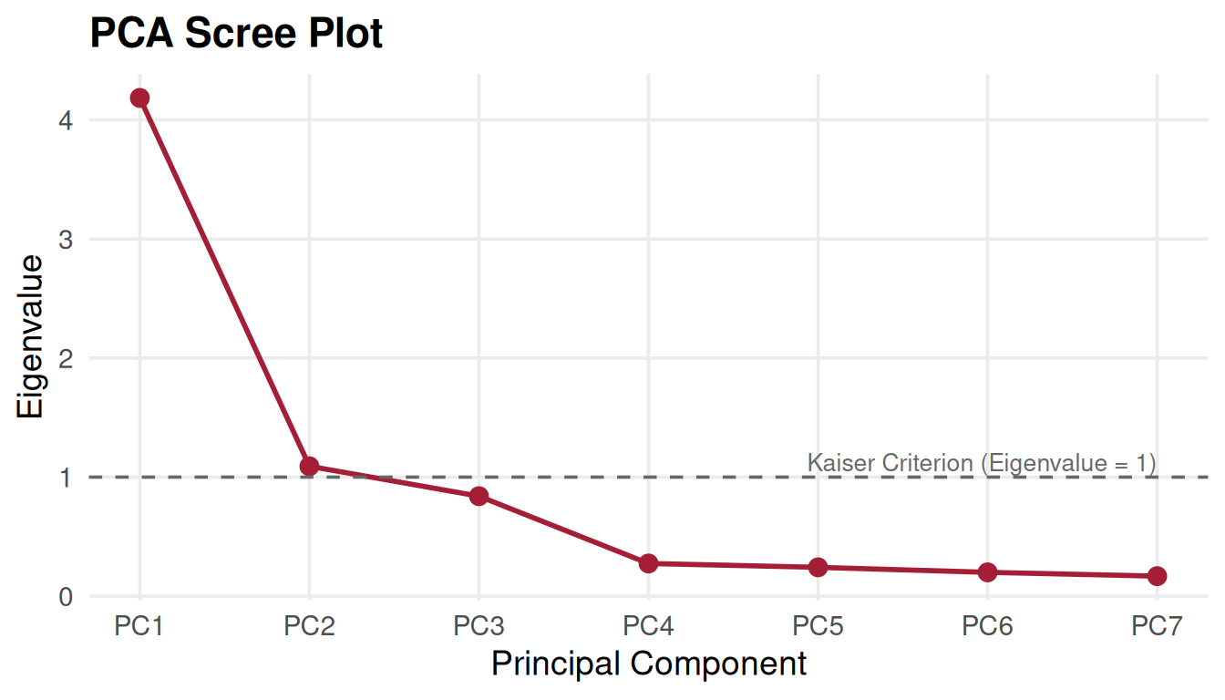

pca_variables_plot(clin_pca, title = "Clinical Variable Correlations with PC1 and PC2")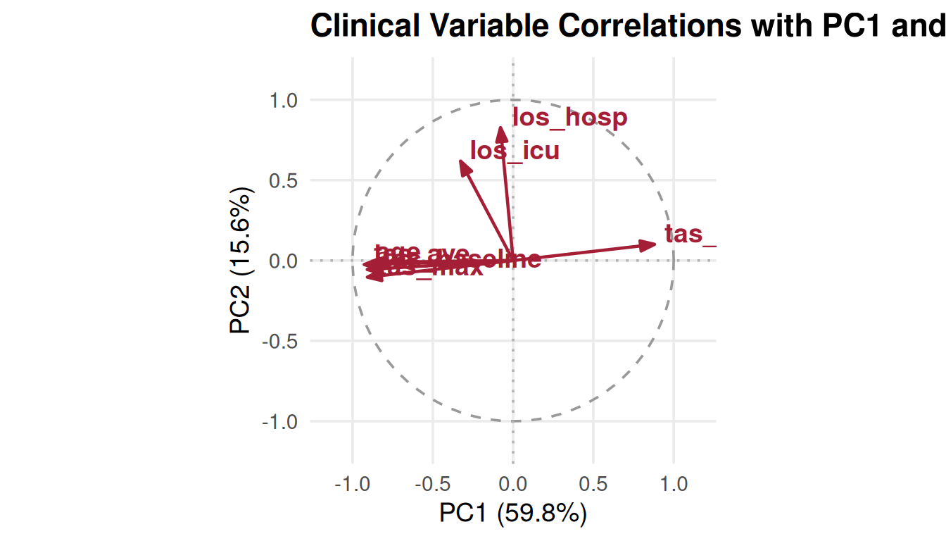

Examining Variable Loadings (Eigenvectors)

rotation_matrix(attr(clin_pca, "prcomp"))[, c("feature", "PC1", "PC2", "PC3")]
#> # A tibble: 7 × 4
#>   feature          PC1     PC2      PC3
#>   <chr>          <dbl>   <dbl>    <dbl>
#> 1 age          -0.433  -0.0113  0.0179 
#> 2 tas_baseline -0.444  -0.0538 -0.0675 
#> 3 tas_min       0.430   0.0962  0.157  
#> 4 tas_max      -0.444  -0.0993 -0.0301 
#> 5 tas_ave      -0.453  -0.0241  0.00513
#> 6 los_icu      -0.160   0.592   0.775  
#> 7 los_hosp     -0.0384  0.792  -0.607

Connecting PCA to Multivariable Cox Survival Modeling

In Darina Chudnovskaya’s applied research, univariable Cox regression showed that physiological indicators (tas_baseline, tas_min, tas_max, tas_ave, age) were statistically significant predictors of survival, whereas length of stay metrics (los_icu, los_hosp) primarily reflected post-admission hospital course:

Collinearity Identification: tas_min, tas_max, and tas_ave cluster tightly in loading space. Entering all three simultaneously into a multivariable Cox model (cox_multi()) inflates variance and causes coefficient instability.
Dimension Separation: PCA isolates the hospital stay duration axis ( $PC_1$ ) from acute physiological thermal volatility ( $PC_2$ and $PC_3$ ).
Model Selection Guidance: In conjunction with univariable tables (cox_single()) and baseline summaries (summary_table()), PCA provides empirical justification for retaining a single representative metric (such as tas_ave or tas_baseline) or constructing an orthogonal composite score.

SAS PROC PRINCOMP to TempleCBE Translation Guide

The table below summarizes common SAS PROC PRINCOMP statements and options alongside their TempleCBE equivalents:

Task / Feature	SAS `PROC PRINCOMP` Syntax	`TempleCBE` Syntax
Fit Standardized PCA	`proc princomp data=mydata; var x1-x10; run;`	`run_pca(mydata, scale = TRUE)`
Unstandardized (Covariance) PCA	`proc princomp data=mydata cov; run;`	`run_pca(mydata, scale = FALSE)`
Output PC Scores to Dataset	`proc princomp data=mydata out=pca_scores; run;`	`predict(attr(res, "prcomp"), mydata)`
Scree Plot	`proc princomp plots=scree; run;`	`pca_scree_plot(res, kaiser = TRUE)`
Biplot	`proc princomp plots=biplot; run;`	`pca_biplot(res, group = group_vec, ellipse = TRUE)`
Variable Correlation Plot	`proc princomp plots=pattern; run;`	`pca_variables_plot(res)`
Feature Loading Heatmap	(SAS Graph Template required)	`pca_plot(res, type = "heatmap")`
Linear Combination Equations	(Manual calculation in DATA step)	`pca_eqns(attr(res, "prcomp"))`
Compare Fits Across Cohorts	(Manual matrix subtraction)	`pca_loading_diff(fit_a, fit_b)`

References

Chudnovskaya, D. (2025). Principal Component Analysis in R and SAS. Biostatistics Technical Report & Lecture Series, Temple University College of Public Health / Lewis Katz School of Medicine.
Jolliffe, I. T., & Cadima, J. (2016). Principal component analysis: a review and recent developments. Philosophical Transactions of the Royal Society A: Mathematical, Physical and Engineering Sciences, 374(2065), 20150202.
SAS Institute Inc. (2023). SAS/STAT User’s Guide: The PRINCOMP Procedure. Cary, NC: SAS Institute Inc.
Built In. A Step-by-Step Explanation of Principal Component Analysis. https://builtin.com/data-science/step-step-explanation-principal-component-analysis
UCLA Statistical Consulting Group. Principal Components Analysis in SAS. https://stats.oarc.ucla.edu/sas/output/principal-components-analysis/