PCA Variable Correlation Circle

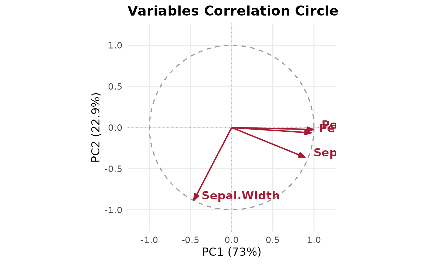
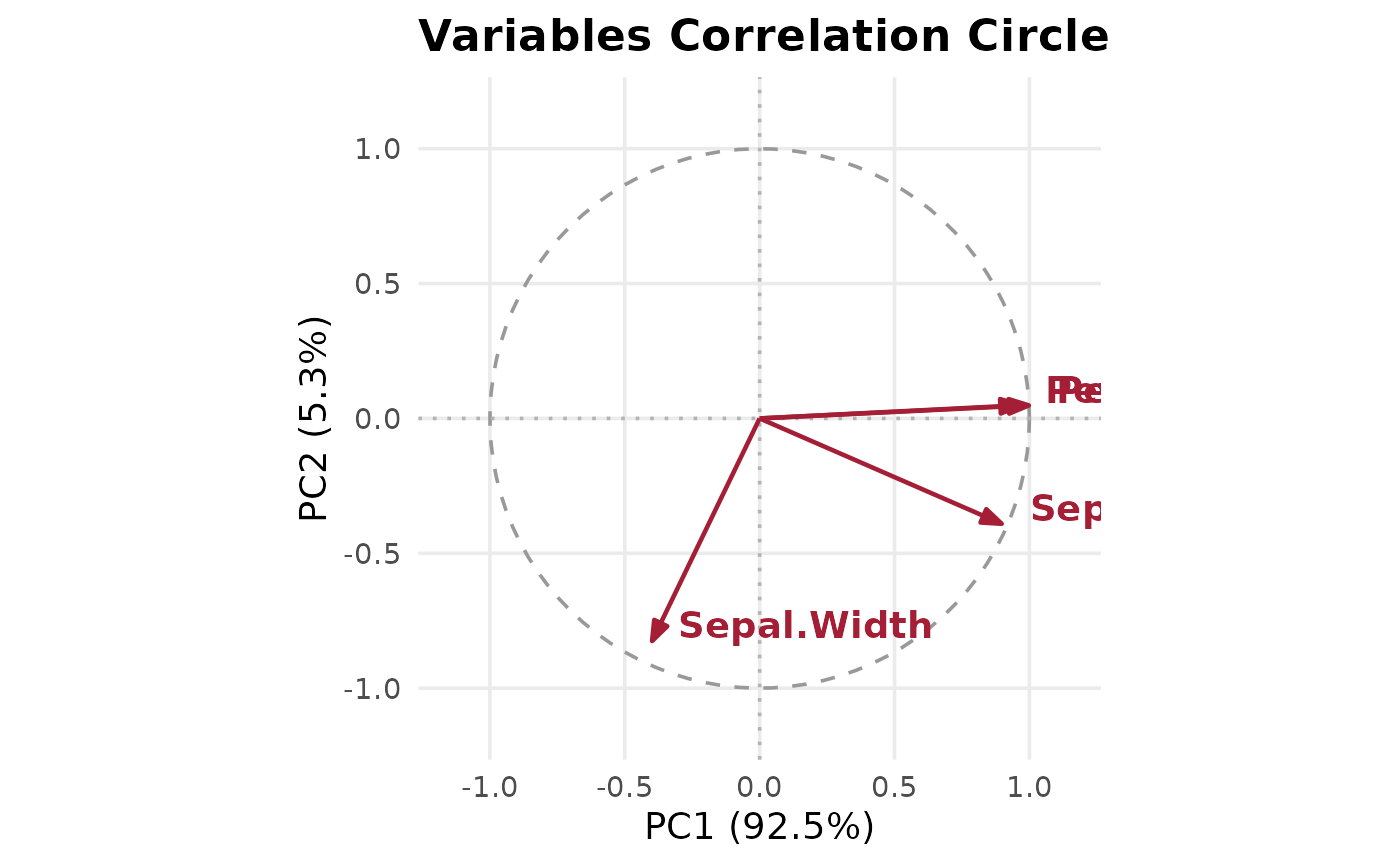
Plots the projection of variables onto the unit circle for two principal components, showing correlations between original variables and principal components.

Usage

pca_variables_plot(
  pca_model,
  x = 1,
  y = 2,
  title = "Variables Correlation Circle",
  data = NULL
)

Arguments

pca_model

A prcomp object or output from run_pca.

x, y

Which principal components to plot (default 1, 2).

title

Optional plot title (default "Variables Correlation Circle").

data

Optional data frame or matrix holding the original variables (numeric, with a column for each variable of pca_model, matched by name). When given, the arrows show cor(data, scores), the correlations between the variables and the component scores of data, whatever the scaling of pca_model, and the unscaled warning is not given. Default NULL: loading times standard deviation.

Value

A ggplot object.

Details

Each arrow ends at the variable's loading times the component's standard deviation. For a PCA of standardised variables (prcomp(scale. = TRUE), a correlation-matrix PCA) that is the correlation between the variable and the component, so every arrow lies inside the unit circle. For a PCA of unscaled variables (the prcomp default, scale. = FALSE) it is a covariance in the units of the data, which can exceed 1, and the function warns. A prcomp object does not keep the data it was fit to, so either refit with prcomp(scale. = TRUE) or give the original variables as data, which computes the correlations directly.

Fits truncated with rank. or tol are supported: the percent of variance on the axis labels is still the share of the total variance.

Examples

pca_model <- prcomp(iris[, 1:4], center = TRUE, scale. = TRUE)
pca_variables_plot(pca_model)


# An unscaled PCA needs the data to draw correlations.
pca_unscaled <- prcomp(iris[, 1:4])
pca_variables_plot(pca_unscaled, data = iris[, 1:4])