02. Penalized Cox Models and Nested Cross-Validation for Start/Stop Survival Data

Why start/stop data needs care

In counting-process (start/stop) layout, each subject has one row per interval, Surv(tstart, tstop, status), so covariates can change over follow-up. Three things go wrong if those rows are treated as independent observations:

Resampling leaks. Row-level folds, like those of glmnet::cv.glmnet(), put some of a subject’s intervals in the analysis set and others in the assessment set.
Scoring is wrong, silently. yardstick’s survival metrics expect one row per subject with right-censored truth. Given start/stop truth, they return numbers without complaint, but those numbers count every interval as its own subject.
Censoring is ignored. Brier scores need inverse-probability-of-censoring weights, or subjects lost to follow-up bias the score.

TempleCBE handles each of these:

Function	What it does
`coxnet()`	Elastic-net Cox model (glmnet) with formula, recipe, and x/y interfaces (hardhat)
`cv_coxnet()`	Chooses `mixture` and `penalty` on subject-grouped folds with a yardstick metric set
`nested_cv_coxnet()`	Estimates how well that whole tuning procedure generalizes
`surv_subject_truth()`, `censoring_km()`, `graf_weights()`, `add_graf_weights()`	Score any start/stop model with yardstick

Comparison with existing R survival & modeling ecosystems

Survival analysis and prognostic modeling in R are supported by several foundational packages, including survival, glmnet, tidymodels (censored, yardstick), and specialized evaluation packages like pec and survAUC. However, applying these frameworks to real-world clinical cohorts with longitudinal visits, time-dependent covariates, and multi-center structures reveals substantial hurdles:

Existing tools and their limitations in longitudinal clinical modeling

survival (Therneau): The foundational baseline for semi-parametric Cox proportional hazards and Kaplan-Meier estimation. While excellent for classical low-dimensional epidemiological inference, it lacks high-dimensional regularization (lasso, elastic net), automated cross-validation, and tidy resampling integration.
glmnet::cv.glmnet(family = "cox") (Friedman et al.): The standard penalized Cox implementation. However:
- Data leakage on start/stop data: cv.glmnet constructs folds by randomly partitioning individual rows. In counting-process data (Surv(tstart, tstop, status)), this splits intervals belonging to the same patient across training and validation folds, leaking patient identity and future biomarker trajectory into the validation set.
- No cluster/site-level grouping: It cannot hold out entire clinical sites or hospital clusters to evaluate generalizability across centers.
- Suboptimal metric selection: It chooses the penalty parameter $\lambda$ using partial likelihood deviance or Harrell’s C-index, without support for time-dependent calibration, Integrated Brier Scores (IBS), or IPCW adjustments.
- No modern formula/recipe preprocessing: Predictors must be supplied as a raw numeric design matrix ( $x$ ), forcing manual one-hot encoding outside the cross-validation loop.
tidymodels / censored / yardstick: The modern tidy modeling framework. While censored bridges parsnip to survival models, its longitudinal counting-process support remains limited:
- Silent scoring failures: yardstick survival metrics expect one row per subject with right-censored truth (Surv(time, event)). When provided with counting-process intervals (Surv(tstart, tstop, event)), yardstick returns numbers without error, but silently treats every interval as an independent patient, biasing both Brier scores and ROC AUCs.
- Missing integrated nested CV for penalized Cox: Evaluating regularized Cox models across an $\alpha$ -mixture and $\lambda$ -penalty grid with subject-level IPCW weights requires bespoke orchestration.
pec / riskRegression / survAUC: Provide inverse-probability-of-censoring weights and prediction error curves, but operate as standalone legacy systems decoupled from recipes preprocessing and the tidymodels grammar.

Where `TempleCBE` provides distinct value

TempleCBE unifies high-dimensional regularization, tidy recipes, and rigorous counting-process survival theory into an integrated, leak-free pipeline:

Strict patient- and site-grouped resampling: cv_coxnet() and nested_cv_coxnet() enforce grouping by patient (group = "patient_id") or site (group = "site"), guaranteeing that all longitudinal intervals for a patient stay within either the analysis set or the assessment set.
Formal start/stop to subject-truth translation: surv_subject_truth() collapses multi-interval records into the valid single-row-per-subject truth required by yardstick, verifying that intervals do not overlap and that events occur only at terminal visits.
Inverse-probability-of-censoring (Graf) weighting: censoring_km(), graf_weights(), and add_graf_weights() estimate the reverse Kaplan-Meier censoring distribution on the training set and attach time-dependent IPCW weights to test predictions, ensuring Brier scores and ROC curves remain unbiased.
True nested cross-validation: nested_cv_coxnet() optimizes hyperparameters strictly on inner folds and scores untouched outer assessment folds, delivering an honest estimate of clinical generalizability.
Mixed continuous and categorical feature spaces: Through step_famd(), TempleCBE integrates Factor Analysis of Mixed Data directly into recipes, allowing joint dimensionality reduction across continuous clinical labs and discrete clinical stages.
Translational laboratory export: km_summary_to_prism() translates survival curves into GraphPad Prism-compatible format for oncology and pharmacology deliverables.

Feature comparison matrix

Dimension	`survival`	`glmnet::cv.glmnet`	`tidymodels` (native)	`TempleCBE`
Counting-process (`tstart, tstop`)	Full support	Partial (leaks rows in CV)	Limited in `censored`	Full leak-free support
Resampling grouping	Manual	No (row-level only)	`group_vfold_cv()`	Native patient & site grouping
Penalty selection metric	None (unpenalized)	Deviance or Concordance	Depends on metric set	Time-dependent IBS & Concordance
IPCW adjustment for start/stop	Manual	None	Silent row-level miscount	Automated via `graf_weights()`
Tidy recipes integration	None	None	Standard recipes	Full `recipes` + `step_famd()`
Nested cross-validation engine	None	None	Manual multi-loop script	Automated via `nested_cv_coxnet()`
Mixed-data dimensionality reduction	None	None	`step_pca` (numeric only)	`step_famd` (mixed continuous/discrete)
GraphPad Prism deliverable export	None	None	None	Built-in via `km_summary_to_prism()`

Specific operational and statistical gaps addressed

1. Resampling leakage in longitudinal patient cohorts

In clinical studies tracking chronic disease (e.g. cardiovascular disease, oncology, sepsis in the ICU), patients undergo repeated visits with drifting biomarkers. When penalized models are cross-validated at the row level, a model trained on visit 1 and visit 3 is tested on visit 2 of the same patient. This produces artificially deflated prediction error and false optimism. TempleCBE guarantees zero leakage across all cross-validation stages.

2. Silent metric bias in counting-process evaluation

Standard evaluation metrics assume each observation corresponds to one independent individual. Scoring longitudinal intervals directly artificially inflates sample size (e.g. 150 patients with 4 visits each scored as 600 independent patients) and ignores informative censoring. TempleCBE provides the necessary mathematical transformations (surv_subject_truth() + graf_weights()) so that yardstick evaluates patients properly.

3. High-dimensional clinical feature reduction for mixed data

Clinical prediction models frequently ingest hundreds of variables combining continuous laboratory biomarkers with categorical ICD-10 diagnostic codes, cancer stages, and medication history. Standard PCA cannot handle categorical variables without arbitrary one-hot expansion that distorts covariance. TempleCBE::step_famd() provides mathematically principled dimensionality reduction for mixed data within standard tidymodels workflows.

library(TempleCBE)
library(tidymodels)
library(survival)
tidymodels_prefer()

Simulated data

Each patient has one to four visits at irregular times, belongs to one of five sites, and has a marker that drifts between visits. An event can only occur in a patient’s last interval.

set.seed(42)
sim_data <- purrr::map(seq_len(150), function(i) {
  n_visits <- sample(1:4, 1)
  tstop <- round(cumsum(runif(n_visits, 20, 40)))
  age <- rnorm(1, mean = 58, sd = 10)
  treatment <- sample(c("Control", "Treated"), 1)
  marker <- rnorm(1) + cumsum(rnorm(n_visits, sd = 0.3))
  risk <- 0.03 * (age - 58) + 0.8 * marker[n_visits] - 0.6 * (treatment == "Treated")
  tibble(
    patient_id = sprintf("PT_%03d", i),
    site = paste0("site_", i %% 5 + 1),
    tstart = c(0, head(tstop, -1)),
    tstop = tstop,
    status = c(rep(0L, n_visits - 1), rbinom(1, 1, plogis(risk))),
    age = age,
    bmi = rnorm(1, mean = 27, sd = 4),
    marker = marker,
    treatment = factor(treatment, levels = c("Control", "Treated"))
  )
}) |>
  purrr::list_rbind()

sim_data
#> # A tibble: 362 × 9
#>    patient_id site   tstart tstop status   age   bmi marker treatment
#>    <chr>      <chr>   <dbl> <dbl>  <int> <dbl> <dbl>  <dbl> <fct>    
#>  1 PT_001     site_2      0    39      0  52.4  26.6 -0.283 Treated  
#>  2 PT_002     site_3      0    25      0  78.2  26.5 -0.174 Treated  
#>  3 PT_002     site_3     25    54      0  78.2  26.5  0.310 Treated  
#>  4 PT_002     site_3     54    93      0  78.2  26.5  0.321 Treated  
#>  5 PT_003     site_4      0    36      0  67.7  28.2  1.23  Treated  
#>  6 PT_003     site_4     36    64      0  67.7  28.2  0.694 Treated  
#>  7 PT_003     site_4     64    98      0  67.7  28.2  0.642 Treated  
#>  8 PT_003     site_4     98   118      0  67.7  28.2  1.01  Treated  
#>  9 PT_004     site_5      0    28      1  65.9  35.5  0.268 Treated  
#> 10 PT_005     site_1      0    37      0  51.9  17.3 -1.03  Treated  
#> # ℹ 352 more rows

Collapsed to one row per patient, this is the truth yardstick needs:

surv_subject_truth(Surv(sim_data$tstart, sim_data$tstop, sim_data$status), sim_data$patient_id)
#> # A tibble: 150 × 3
#>    .subject_id .entry .truth
#>    <chr>        <dbl> <Surv>
#>  1 PT_001           0    39+
#>  2 PT_002           0    93+
#>  3 PT_003           0   118+
#>  4 PT_004           0    28 
#>  5 PT_005           0    61+
#>  6 PT_006           0    20+
#>  7 PT_007           0    20 
#>  8 PT_008           0    28 
#>  9 PT_009           0    51 
#> 10 PT_010           0    38+
#> # ℹ 140 more rows

Fitting one model: `coxnet()`

coxnet() fits the whole glmnet regularization path. The formula interface expands factors into indicator columns.

fit <- coxnet(
  Surv(tstart, tstop, status) ~ age + bmi + marker + treatment,
  data = sim_data, mixture = 0.5, penalty = 0.01
)
fit
#> <coxnet_model> penalized Cox model (start/stop outcome)
#>   rows: 362  predictors: 5  events: 65 
#>   mixture: 0.5  penalties on path: 64 
#>   default penalty: 0.01
tidy(fit)
#> # A tibble: 5 × 3
#>   term             estimate penalty
#>   <chr>               <dbl>   <dbl>
#> 1 age               0          0.01
#> 2 bmi               0.0184     0.01
#> 3 marker            0.257      0.01
#> 4 treatmentControl  0          0.01
#> 5 treatmentTreated -0.00531    0.01

Predictions follow tidymodels conventions: .pred_linear_pred (larger means longer survival), or a .pred list-column of survival probabilities.

predict(fit, sim_data[1:3, ], type = "survival", eval_time = c(30, 60, 90))$.pred[[1]]
#> # A tibble: 3 × 2
#>   .eval_time .pred_survival
#>        <dbl>          <dbl>
#> 1         30          0.945
#> 2         60          0.821
#> 3         90          0.649

Choosing `mixture` and `penalty`: `cv_coxnet()`

With a recipe, preprocessing is learned inside each fold. The outcome is a Surv column; the patient identifier gets the "id" role, which cv_coxnet() uses to group folds and score patients.

sim_data$surv <- Surv(sim_data$tstart, sim_data$tstop, sim_data$status)

cox_rec <- recipe(surv ~ age + bmi + marker + treatment + patient_id + site, data = sim_data) |>
  update_role(patient_id, new_role = "id") |>
  update_role(site, new_role = "site") |>
  step_dummy(treatment) |>
  step_normalize(all_numeric_predictors())

set.seed(2026)
cv <- cv_coxnet(cox_rec, sim_data, mixture = c(0.25, 0.5, 1), v = 5, nlambda = 30)
cv
#> <cv_coxnet> penalized Cox model, 5 resamples
#>   metric: brier_survival_integrated (minimize)  
#>   mixture: 0.5   lambda.min: 0.06337   lambda.1se: 0.1196 
#>   mean at lambda.min: 0.1414 (std. error 0.00739)

By default every fold is scored with the integrated Brier score (used to choose), concordance, and the time-specific Brier score and ROC AUC, at deciles of the observed event times.

collect_metrics(cv) |>
  filter(.metric %in% c("brier_survival_integrated", "concordance_survival")) |>
  arrange(.metric, mean)
#> # A tibble: 114 × 8
#>    mixture penalty .metric             .estimator .eval_time  mean     n std_err
#>      <dbl>   <dbl> <chr>               <chr>           <dbl> <dbl> <int>   <dbl>
#>  1    0.5   0.0634 brier_survival_int… standard           NA 0.141     5 0.00739
#>  2    0.25  0.127  brier_survival_int… standard           NA 0.141     5 0.00748
#>  3    1     0.0317 brier_survival_int… standard           NA 0.141     5 0.00734
#>  4    0.25  0.0923 brier_survival_int… standard           NA 0.141     5 0.00756
#>  5    0.5   0.0461 brier_survival_int… standard           NA 0.142     5 0.00757
#>  6    1     0.0435 brier_survival_int… standard           NA 0.142     5 0.00732
#>  7    0.5   0.0871 brier_survival_int… standard           NA 0.142     5 0.00743
#>  8    0.25  0.174  brier_survival_int… standard           NA 0.142     5 0.00757
#>  9    1     0.0231 brier_survival_int… standard           NA 0.142     5 0.00762
#> 10    0.25  0.0672 brier_survival_int… standard           NA 0.142     5 0.00775
#> # ℹ 104 more rows
autoplot(cv)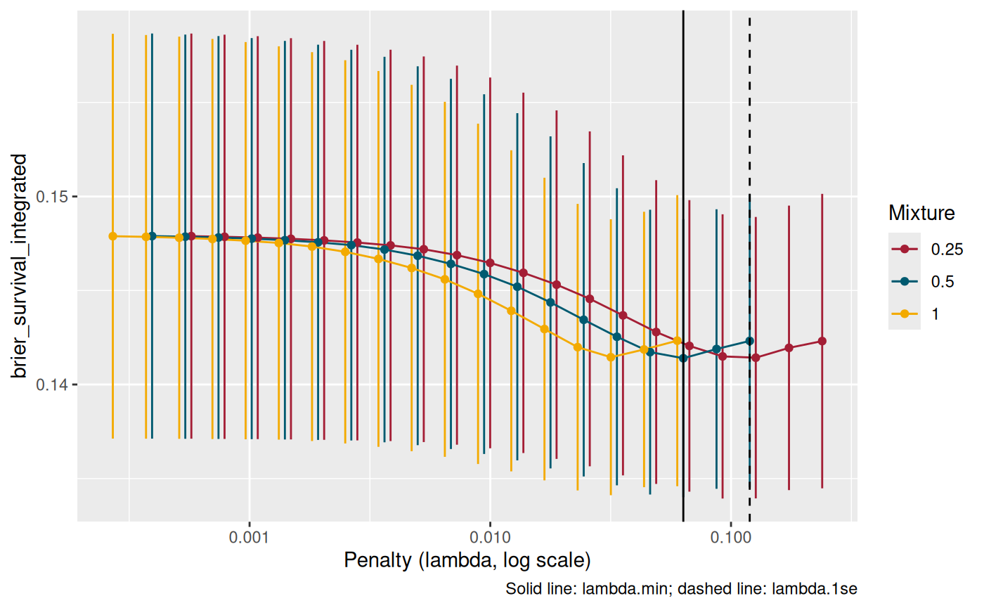

tidy(cv, penalty = "lambda.1se")
#> # A tibble: 4 × 3
#>   term              estimate penalty
#>   <chr>                <dbl>   <dbl>
#> 1 age                      0   0.120
#> 2 bmi                      0   0.120
#> 3 marker                   0   0.120
#> 4 treatment_Treated        0   0.120

Folds can be grouped by a coarser unit than the patient. With group = "site", each fold holds out whole sites:

set.seed(2026)
cv_sites <- cv_coxnet(
  cox_rec, sim_data, group = "site", v = 5, nlambda = 20,
  metrics = metric_set(brier_survival_integrated, concordance_survival)
)
cv_sites$best_by_mixture
#> # A tibble: 1 × 5
#>   mixture lambda_min lambda_1se  mean std_err
#>     <dbl>      <dbl>      <dbl> <dbl>   <dbl>
#> 1       1     0.0368     0.0598 0.142  0.0144

How well does tuning generalize? `nested_cv_coxnet()`

A cross-validated score at the chosen settings is optimistic: the same assessment sets chose the settings. Nested cross-validation tunes on inner resamples, refits on each outer analysis set, and scores the untouched outer assessment set.

set.seed(2026)
nested_folds <- nested_cv(
  sim_data,
  outside = group_vfold_cv(group = patient_id, v = 3),
  inside = group_vfold_cv(group = patient_id, v = 3)
)

nested <- nested_cv_coxnet(
  nested_folds, cox_rec,
  mixture = c(0.5, 1), rule = "1se", nlambda = 20,
  metrics = metric_set(brier_survival_integrated, concordance_survival)
)
nested |> select(id, mixture, penalty)
#> # A tibble: 3 × 3
#>   id        mixture penalty
#>   <chr>       <dbl>   <dbl>
#> 1 Resample1     0.5  0.144 
#> 2 Resample2     1    0.0612
#> 3 Resample3     0.5  0.0903
collect_metrics(nested)
#> # A tibble: 2 × 6
#>   .metric                   .estimator .eval_time  mean     n std_err
#>   <chr>                     <chr>           <dbl> <dbl> <int>   <dbl>
#> 1 brier_survival_integrated standard           NA 0.143     3 0.00922
#> 2 concordance_survival      standard           NA 0.544     3 0.00543

Scoring any start/stop model with yardstick

The same helpers score predictions from any model. Here, a coxnet() fit predicts each test patient’s survival from their baseline covariates:

set.seed(2026)
split <- group_initial_split(sim_data, group = patient_id)
train <- training(split)
test <- testing(split)
times <- c(30, 60, 90)

model <- coxnet(
  Surv(tstart, tstop, status) ~ age + bmi + marker + treatment,
  data = train, mixture = cv$mixture, penalty = cv$lambda_min
)

train_truth <- surv_subject_truth(train$surv, train$patient_id)
test_truth <- surv_subject_truth(test$surv, test$patient_id)
baseline_rows <- test |> filter(tstart == 0) |> arrange(patient_id)

scored <- test_truth |>
  bind_cols(predict(model, baseline_rows, type = "survival", eval_time = times)) |>
  add_graf_weights(censoring = censoring_km(train_truth$.truth))

brier_survival_integrated(scored, truth = .truth, .pred)
#> # A tibble: 1 × 3
#>   .metric                   .estimator .estimate
#>   <chr>                     <chr>          <dbl>
#> 1 brier_survival_integrated standard       0.121

Existing analysis code: `glmnet_IBS()`

glmnet_IBS(), tune_over_alpha(), and tune_alpha_by_split() keep their arguments. They now use cv_coxnet() underneath, so the penalty is chosen on patient-grouped folds and the IBS uses censoring weights.

legacy_rec <- recipe(~ age + bmi + marker + treatment + patient_id + tstart + tstop + status, data = sim_data) |>
  update_role(patient_id, tstart, tstop, status, new_role = "id variable") |>
  step_dummy(treatment) |>
  step_normalize(all_numeric_predictors())

set.seed(2026)
glmnet_IBS(
  split, alpha = 0.5, recipe = legacy_rec,
  feature_names = c("age", "bmi", "marker", "treatment_Treated"),
  eval_time = times, id_col = "patient_id", internal_folds = 3
)
#> # A tibble: 4 × 5
#>     IBS lambda term              estimate alpha
#>   <dbl>  <dbl> <chr>                <dbl> <dbl>
#> 1 0.121  0.101 age                 0        0.5
#> 2 0.121  0.101 bmi                 0        0.5
#> 3 0.121  0.101 marker              0.0689   0.5
#> 4 0.121  0.101 treatment_Treated   0        0.5

Highlighting core TempleCBE survival and modeling utilities

Beyond the core coxnet() modeling functions, TempleCBE includes several specialized utilities that address frequent friction points in biostatistical practice:

1. Mixed-data dimensionality reduction with `step_famd()`

Clinical prognostic modeling frequently involves datasets with dozens of continuous lab values (e.g. creatinine, bilirubin, blood pressure) alongside categorical clinical indicators (e.g. disease stage, smoking status, sex, treatment center). Standard Principal Component Analysis ([recipes::step_pca()]) only operates on numeric columns; dummy-encoding categorical variables before PCA distorts the geometric distances because binary indicators have different variances than continuous variables.

step_famd() provides a native recipes step for Factor Analysis of Mixed Data (Pagès 2004, implemented via FactoMineR::FAMD): - Continuous variables are normalized to unit variance. - Categorical variables are dummy-coded and weighted inversely by their category frequencies, ensuring each variable contributes proportionally regardless of its number of levels.

library(recipes)

# Define clinical recipe with mixed numeric and categorical predictors
mixed_rec <- recipe(surv ~ age + bmi + marker + treatment + site + patient_id, data = sim_data) |>
  update_role(patient_id, new_role = "id") |>
  # Apply FAMD to compress continuous and discrete predictors into 3 components
  step_famd(age, bmi, marker, treatment, site, num_comp = 3, prefix = "FAMD_")

# Train and inspect component contributions
prepped_famd <- prep(mixed_rec, training = sim_data)
baked_features <- bake(prepped_famd, new_data = NULL)
head(baked_features)

# Inspect variance explained by components
tidy(prepped_famd, number = 1, type = "variance")

step_famd() integrates directly into cv_coxnet() and nested_cv_coxnet(), ensuring that components are learned strictly inside each training fold without leakage.

2. Framework-agnostic survival scoring with `surv_helpers`

The helper functions in surv_helpers.R are not restricted to coxnet(): they enable any model (e.g. random survival forests via ranger, gradient boosted survival trees via xgboost, or deep learning survival models) to be properly evaluated on longitudinal start/stop cohorts using yardstick:

surv_subject_truth(): Collapses start/stop interval data to a single row per patient with right-censored truth.
censoring_km(): Estimates the reverse Kaplan-Meier censoring distribution $\hat{G}(t) = P(C > t)$ on the training cohort.
graf_weights() / add_graf_weights(): Adds Inverse Probability of Censoring Weights (Graf et al. 1999) to prediction tibbles.

# Scoring any external model predictions on test subjects:
test_truth <- surv_subject_truth(test_longitudinal$surv, test_longitudinal$patient_id)
train_censoring <- censoring_km(train_subject_truth$.truth)

# Combine test truth with external model predictions and add IPCW weights
scored_predictions <- test_truth |>
  bind_cols(external_model_predictions) |>
  add_graf_weights(censoring = train_censoring)

# Compute proper, unbiased integrated Brier score
yardstick::brier_survival_integrated(scored_predictions, truth = .truth, .pred)

3. Distributed elastic net tuning with `survival_metrics`

When searching over a broad grid of elastic net mixing parameters ( $\alpha$ ) or evaluating competing candidate clinical formulas, tune_over_alpha(), tune_alpha_by_split(), and score_outer() orchestrate parallel evaluation using furrr.

Nested Parallelism & Cluster Benchmarking Architecture

In nested survival cross-validation, total computational workload scales multiplicatively: $\text{Total Fits} = N_{\text{outer folds}} \times N_{\text{inner splits}} \times N_{\alpha \text{ values}} \times N_{\text{internal CV folds}}$

For example, a study with 7 outer folds, 7 inner resamples, 10 candidate $\alpha$ mixing parameters, and 5 internal penalty selection folds requires $7 \times 7 \times 10 \times 5 = 2,450$ penalized Cox model estimations per clinical domain.

Best Practices for Cluster & Multicore Execution: 1. Outer/Split Parallelism: Set future::plan(multisession, workers = N) at the session level before invoking tuning or scoring. TempleCBE functions strictly adhere to the never call plan() inside functions fleet rule. 2. Sequential Inner Fits: Avoid setting parallel = TRUE inside glmnet_IBS() when tune_alpha_by_split() is already running across parallel workers; nested socket clusters lead to worker resource contention and OS deadlocks. 3. Resilience with Checkpoints: Pass checkpoint_dir = "checkpoints/tuning_abg" to tune_alpha_by_split(), tune_over_alpha(), and score_outer(). Completed tasks save atomic .rds artifacts per split/fold. If a run is interrupted across cluster nodes, rerunning detects cached checkpoints and skips recomputation with an informative progress notice. 4. Environment Isolation: Multisession worker processes automatically import required preprocessing namespaces (recipes, rsample, yardstick, survival, glmnet).

library(furrr)
plan(multisession, workers = 4)

# Parallel grid search across alpha values with checkpointing
alpha_results <- tune_over_alpha(
  split,
  recipe = cox_rec,
  num_alpha_values = 10,
  internal_folds = 5,
  progress = TRUE,
  checkpoint_dir = "checkpoints/alpha_grid"
)

# Summarize results across all inner splits of a nested resample
nested_alpha_summary <- tune_alpha_by_split(
  nested_folds$inner_resamples[[1]],
  checkpoint_dir = "checkpoints/inner_splits",
  progress = TRUE
)

4. Translating survival curves to GraphPad Prism with `km_summary_to_prism()`

In academic medical centers, biostatisticians frequently collaborate with laboratory scientists, pharmacologists, and clinical trialists who require Kaplan-Meier survival data formatted for GraphPad Prism for manuscript figures and FDA briefing documents.

Prism requires a unique table format: an X column of timepoints, with separate columns per experimental group holding 1 for events, 0 for censored patients, and NA for other groups. km_summary_to_prism() converts standard survival::survfit summary tables directly into this layout:

# Fit standard stratified Kaplan-Meier curve
fit_km <- survfit(Surv(time, status) ~ treatment, data = lung)
km_summary <- summary(fit_km, censored = TRUE)

km_df <- data.frame(
  time     = km_summary$time,
  strata   = km_summary$strata,
  n.risk   = km_summary$n.risk,
  n.event  = km_summary$n.event,
  n.censor = km_summary$n.censor
)

# Convert to GraphPad Prism layout and export to Excel
prism_table <- km_summary_to_prism(
  km_df,
  out_xlsx = "deliverables/Prism_Survival_Table.xlsx"
)
head(prism_table)

How others can use this technology (Adoption Patterns)

Here are five practical adoption patterns for biostatistical and clinical data science teams:

Pattern 1: Longitudinal EHR survival modeling with patient grouping

When modeling electronic health records with repeated clinical visits, replace standard row-level splitting with patient-grouped folds:

# Ensure patient-grouped folds
cv_fit <- cv_coxnet(
  recipe = clinical_rec,
  data = ehr_longitudinal_data,
  group = "patient_id",
  mixture = 0.5,
  v = 5
)

Pattern 2: Mixed clinical & biomarker dimensionality reduction

Combine high-dimensional lab panels and discrete clinical stages using step_famd() inside a tidymodels workflow:

rec <- recipe(surv ~ ., data = cohort) |>
  update_role(patient_id, new_role = "id") |>
  step_famd(all_predictors(), num_comp = 5)

fit <- coxnet(rec, data = cohort, mixture = 1.0, penalty = 0.05)

Pattern 3: Multi-center clinical trial generalizability assessment

Evaluate whether a prognostic signature generalises across hospital sites by grouping cross-validation folds at the institutional site level:

# Hold out entire clinical sites during validation
site_cv <- cv_coxnet(
  recipe = clinical_rec,
  data = multi_site_study,
  group = "hospital_site",
  v = 10,
  metrics = metric_set(brier_survival_integrated, concordance_survival)
)

Pattern 4: Honest generalization auditing with nested cross-validation

Before presenting prognostic scores to clinical stakeholders or submitting models for regulatory evaluation, estimate true out-of-sample generalization using nested_cv_coxnet():

nested_plan <- nested_cv(
  cohort_data,
  outside = group_vfold_cv(group = patient_id, v = 5),
  inside  = group_vfold_cv(group = patient_id, v = 5)
)

honest_metrics <- nested_cv_coxnet(nested_plan, clinical_rec, mixture = c(0.5, 1.0))
collect_metrics(honest_metrics)

Pattern 4b: Honest generalization with inner bootstrap resamples (`group_bootstraps`) vs Random-Alpha exploration

When working with counting-process (start/stop) data where cohort size or event counts are modest, inner grouped bootstraps (group_bootstraps(group = patient_id)) provide smooth, low-variance hyperparameter tuning estimates for choosing $\alpha$ and $\lambda$ :

boot_nested_plan <- nested_cv(
  cohort_data,
  outside = group_vfold_cv(group = patient_id, v = 5),
  inside  = group_bootstraps(group = patient_id, times = 25)
)

honest_boot_metrics <- nested_cv_coxnet(
  boot_nested_plan,
  preprocessor = clinical_rec,
  subject_id = "patient_id",
  mixture = c(0.2, 0.5, 0.8, 1.0)
)
collect_metrics(honest_boot_metrics)

Choosing between Nested Cross-Validation and Random-Alpha Exploration

It is vital to match your statistical strategy to your project question:

Nested Cross-Validation (nested_cv_coxnet):
- Primary Objective: Unbiased generalization performance estimation of the entire modeling strategy.
- How it works: In each outer split, hyperparameters ( $\alpha, \lambda$ ) are optimized solely on inner resamples, refit on the outer analysis set, and scored on held-out outer subjects.
- When to use: Auditing models prior to clinical presentation, benchmarking expected out-of-sample performance, and guarding against optimization bias.
Random-Alpha Hyperparameter Exploration (tune_over_alpha / tune_alpha_by_split):
- Primary Objective: Model selection and diagnostic characterization across the $\alpha \in [0, 1]$ penalty continuum.
- How it works: Evaluates a dense grid or randomized draw of $\alpha$ values across resampling folds, measuring stability, coefficient shrinkage profiles, and Integrated Brier Score sensitivity.
- When to use: Investigating whether Ridge ( $L_2$ ), Lasso ( $L_1$ ), or Elastic Net yields superior feature sparsity and stability, and finalizing a single model specification for deployment.

Pattern 5: Translational laboratory handoff

Seamlessly bridge biostatistical analysis in R with laboratory GraphPad Prism figure creation using km_summary_to_prism():

# Deliver Prism-ready survival spreadsheets to clinical collaborators
km_summary_to_prism(
  km_table,
  out_xlsx = "reports/figures/Figure1_KaplanMeier_Prism.xlsx"
)

Summary

TempleCBE fills the critical gap between classical low-dimensional survival analysis and modern high-dimensional machine learning on longitudinal clinical cohorts. By pairing leak-free grouped resampling (cv_coxnet(), nested_cv_coxnet()) with proper IPCW scoring (surv_helpers), mixed-data feature reduction (step_famd()), and translational handoff tools (km_summary_to_prism()), it provides a robust, reproducible foundation for clinical survival modeling.