04. Validation and Workflow Guide for SAS Users: Cox Models in TempleCBE

J Kyle Armstrong

Introduction: Bridging SAS PROC PHREG and R

In regulated clinical trials and academic biostatistics, SAS PROC PHREG has long been a gold standard for Cox proportional hazards modeling. As modern clinical pipelines increasingly adopt R, biostatisticians and statistical programmers need two critical assurances:

1. Exact Numerical Parity: Confidence that survival models fit in R reproduce the parameter estimates, standard errors, test statistics, and hazard ratios computed by SAS.
2. Workflow Translation: Clear mappings from familiar SAS statements (CLASS, MODEL, BASELINE, ASSESS, OUTPUT) and DATA-step macros to concise, production-ready R workflows.

The TempleCBE package is designed to streamline survival analysis with univariable screening (cox_single()), multivariable modeling (cox_multi()), automated proportional hazards assumption validation (cox_check()), factor reference leveling (relevel_factor()), presentation tables (cbe_cox_table()), and specialized ggplot2 visualizations (plot_cox_forest(), plot_cox_survival(), plot_cox_marginal()).

This vignette demonstrates:

• @sec-part1 — Univariable and multivariable time-fixed survival workflows using the public survival::lung dataset, illustrating SAS-to-R syntax equivalencies.
• @sec-part2 — A formal validation benchmark reproducing SAS Institute’s published results from Example 85.7 (“Time-Dependent Repeated Measurements of a Covariate”), showing numerical concordance to multiple decimal places.
• @sec-part3 — Time-dependent covariate construction comparing the SAS DATA-step macro pattern with survival::tmerge and TempleCBE’s tidy_tmerge_cox().
• @sec-part4 — Model calibration and Integrated Brier Score (IBS) validation with inverse-probability-of-censoring weights (IPCW), comparing TempleCBE to SAS.
• @sec-part5 — Biostatistics Team Entry Point & SAS Macro Suite Guide detailing bundled macros, macro directory access, and execution via run_sas_script().
• @sec-part6 — A comprehensive translation cheat sheet mapping SAS PROC PHREG syntax to TempleCBE.

library(TempleCBE)
library(survival)
library(yardstick)
library(dplyr)
library(ggplot2)

Key Default Differences: SAS vs. R

When validating Cox models between SAS and R, four primary default discrepancies must be kept in mind:

Feature	SAS (PROC PHREG) Default	R (survival::coxph) Default	How to Reconcile in TempleCBE
Tie Handling	TIES=BRESLOW	ties = "efron"	Pass ties = "breslow" into cox_single() or cox_multi().
Factor Coding	Last alphanumeric level is reference unless REF= is specified in CLASS	First factor level is reference	Use relevel_factor() or specify factor levels explicitly.
Baseline Hazards	Centered at covariate means or zeroes via BASELINE	Centered at covariate means in survfit.coxph	Use plot_cox_survival() which handles prediction curves transparently.
Clustered / Repeated Data	ID statement specifies subject grouping	id = ... or cluster(...)	Pass id = ID directly via cox_multi().

Time-Fixed Cox Regression (Public Dataset: survival::lung)

To illustrate the side-by-side syntax without proprietary data, we use the public survival::lung cohort from the North Central Cancer Treatment Group (NCCTG). In survival::lung, the status variable is coded as 1 = censored and 2 = dead. We recode this to standard 0/1 binary status (0 = censored, 1 = dead).

lung_data <- survival::lung %>%
  mutate(
    status = status - 1,
    sex = factor(sex, levels = c(1, 2), labels = c("Male", "Female"))
  )

Univariable Model: Age as a Continuous Predictor

SAS Equivalent

#| lst-label: lst-phreg-univariable
#| lst-cap: "SAS PROC PHREG: Univariable continuous predictor (Breslow ties)"
/* SAS PROC PHREG: Univariable Continuous Model */
proc phreg data=lung;
    model time*status(0) = age / ties=breslow;
run;

TempleCBE Implementation

In TempleCBE, univariable screening is performed with cox_single(). It fits the Cox model, tests the proportional hazards assumption via Schoenfeld residuals, tidies the coefficient table, and generates an automated clinical interpretation:

res_age <- cox_single(
  data = lung_data,
  outcome = "Surv(time, status)",
  feature = "age",
  ties = "breslow"
)

# Clean coefficient table with HR, 95% CI, and formatted p-value
res_age$table
#> # A tibble: 1 × 6
#>   Variable Level           Role         HR `95% CI`    p.value
#>   <chr>    <chr>           <chr>     <dbl> <chr>       <chr>  
#> 1 age      1-unit increase Covariate  1.02 1.00 – 1.04 0.042

The model summary also produces an automated plain-language interpretation:

cat(res_age$interpretation)
#> The hazard ratio for age is 1.02 (95% CI 1 – 1.04). For each one-unit increase in age, the risk of the event increases by 1.9%. The p-value indicates that this association is statistically significant.

And assumption testing is evaluated automatically:

res_age$zph_table
#>            chisq df         p
#> age    0.3434595  1 0.5578391
#> GLOBAL 0.3434595  1 0.5578391
cat(res_age$zph_text)
#> Test of the proportional hazards assumption yields p = 0.558. Therefore, the proportional hazards assumption is not violated.

Univariable Visualizations: Forest, Survival, and Marginal Risk

In SAS, plotting survival curves or marginal effects requires chaining PROC PHREG output with BASELINE statements and PROC SGPLOT. In TempleCBE, one-line functions produce presentation-ready ggplot2 graphics adhering to CBE styling.

Forest Plot

plot_cox_forest(res_age)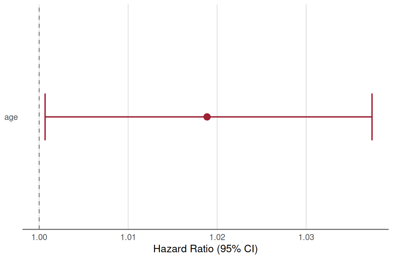

Forest plot of the univariable Cox model for age (hazard ratio with 95% confidence interval).

Survival Curve Overlay

In SAS, one might run:

#| lst-label: lst-phreg-baseline-surv
#| lst-cap: "SAS PROC PHREG + BASELINE + PROC SGPLOT: Predicted survival curve"
proc phreg data=lung;
    model time*status(0) = age / ties=breslow;
    baseline out=pred_surv survival=s / covariates=lung;
run;
proc sgplot data=pred_surv;
    series x=time y=s;
run;

In TempleCBE, plot_cox_survival() plots model-predicted survival curves and can overlay non-parametric Kaplan-Meier curves (overlay_km = TRUE) to visually verify fit adequacy:

plot_cox_survival(res_age, data = lung_data, overlay_km = TRUE)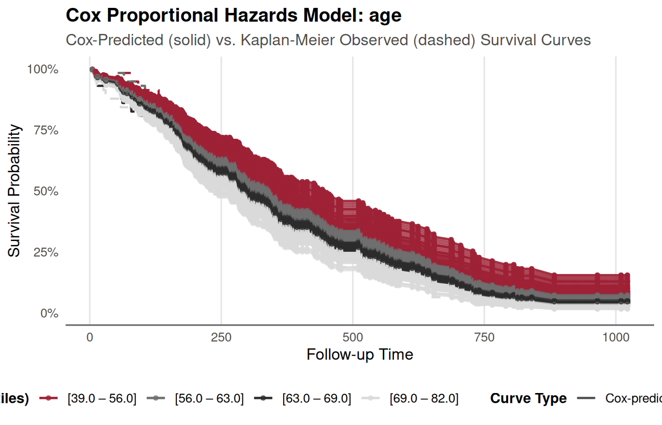

Model-predicted survival curve for the univariable age model, overlaid with the non-parametric Kaplan-Meier estimate.

Marginal Hazard Ratio Curve

To inspect how the relative hazard or mortality probability varies smoothly across the range of the predictor, use plot_cox_marginal():

plot_cox_marginal(res_age, data = lung_data, scale = "hr")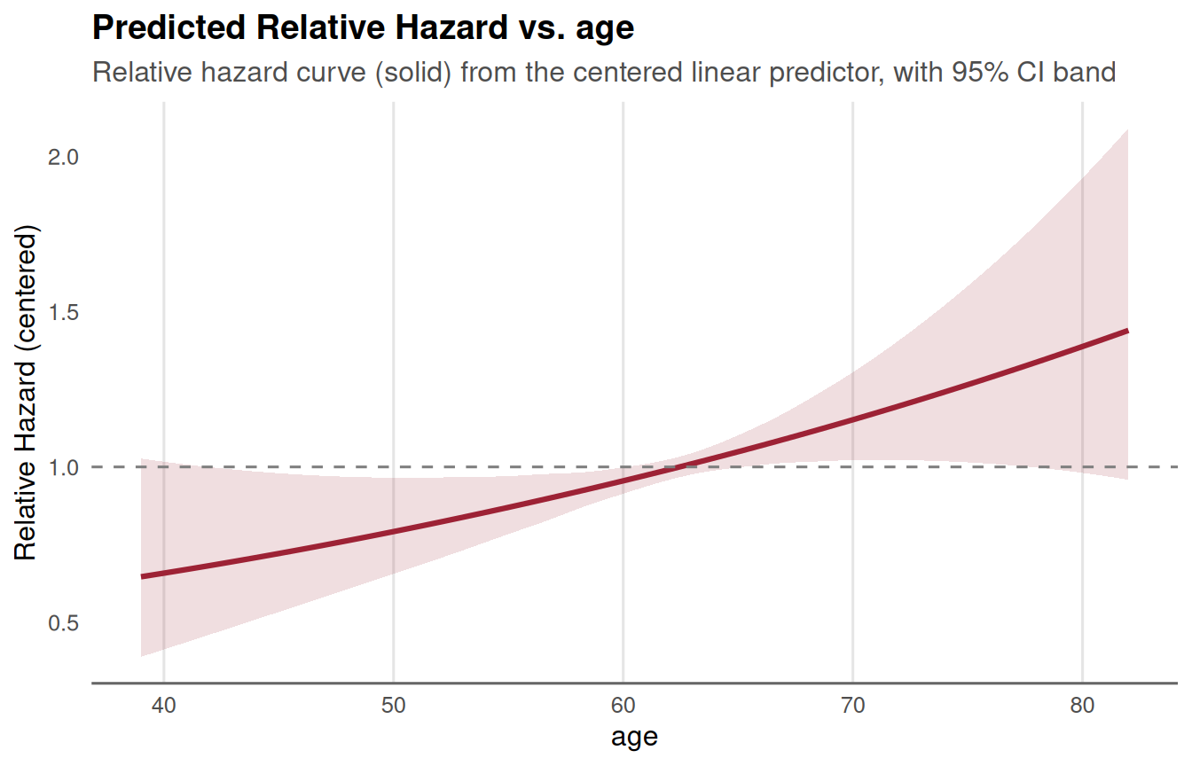

Marginal hazard ratio for age across its observed range, relative to the reference value.

Multivariable Modeling with Categorical Factors

When analyzing multiple predictors, including categorical variables, SAS uses the CLASS statement:

SAS Equivalent

#| lst-label: lst-phreg-multivariable
#| lst-cap: "SAS PROC PHREG: Multivariable model with CLASS reference level"
/* SAS PROC PHREG: Multivariable Model with Reference Level */
proc phreg data=lung;
    class sex(ref="Male") / param=ref;
    model time*status(0) = age sex ph_karno / ties=breslow;
run;

TempleCBE Implementation

In TempleCBE, cox_multi() handles multivariable formulas, supports explicit factor reference rows, and performs both term-specific and global proportional hazards diagnostic checks:

res_multi <- cox_multi(
  data = lung_data,
  formula = Surv(time, status) ~ age + sex + ph.karno,
  ties = "breslow"
)

# Formatted table including explicit reference row for sex = Male
res_multi$table
#> # A tibble: 4 × 7
#>   Variable Level           Role          HR `log(HR)` `95% CI`    p.value
#>   <chr>    <chr>           <chr>      <dbl>     <dbl> <chr>       <chr>  
#> 1 age      1-unit increase Covariate   1.01     0.012 0.99 – 1.03 0.189  
#> 2 sex      Male            Reference   1        0     Reference   —      
#> 3 sex      Female          Comparison  0.61    -0.497 0.44 – 0.85 0.003  
#> 4 ph.karno 1-unit increase Covariate   0.99    -0.013 0.98 – 1.00 0.024

Proportional hazards assumption checks across all terms and the multivariate global test:

res_multi$zph$zph_table
#>               chisq df           p
#> age       0.4766037  1 0.489964719
#> sex       3.0750932  1 0.079500035
#> ph.karno  8.0167557  1 0.004634652
#> GLOBAL   10.3502060  3 0.015812237

Faceted or multi-predictor forest visualization:

plot_cox_forest_multi(res_multi)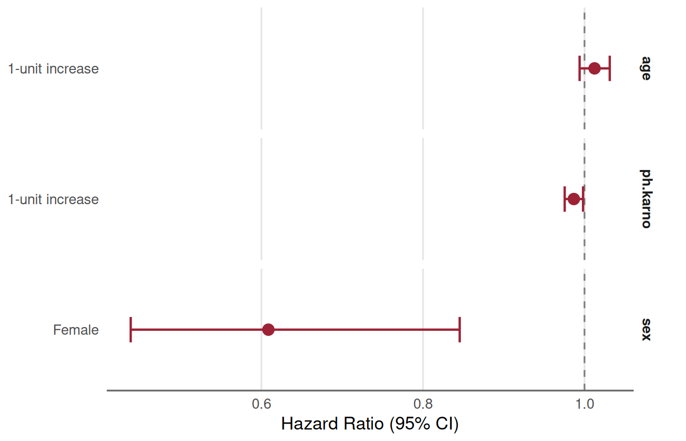

Forest plot of the multivariable Cox model (adjusted hazard ratios with 95% confidence intervals).

And presentation table formatting with global sorting options:

cbe_cox_table(res_multi, sort = "magnitude")
#> # A tibble: 4 × 7
#>   Variable Level           Role          HR `log(HR)` `95% CI`    p.value
#>   <chr>    <chr>           <chr>      <dbl>     <dbl> <chr>       <chr>  
#> 1 sex      Female          Comparison  0.61    -0.497 0.44 – 0.85 0.003  
#> 2 ph.karno 1-unit increase Covariate   0.99    -0.013 0.98 – 1.00 0.024  
#> 3 age      1-unit increase Covariate   1.01     0.012 0.99 – 1.03 0.189  
#> 4 sex      Male            Reference   1        0     Reference   —

Time-Dependent Covariates & Counting Process Benchmark (SAS Example 85.7)

To formally prove numerical equivalence, we implement and validate against SAS/STAT User’s Guide Example 85.7 / 91.7: “Time-Dependent Repeated Measurements of a Covariate”.

Benchmark Study Design

• Cohort: 45 rodents exposed to a carcinogen and randomized to three dose levels of a tumor-promoting agent (Dose: 1.0, 2.5, 10.0).
• Time-Dependent Predictor: Number of papillomas (NPap), observed repeatedly across 15 scheduled observation times (weeks 27, 34, 37, 41, 43, 45, 46, 47, 49, 50, 51, 53, 65, 67, 71).
• Outcome: Death (Dead = 1) or censoring (Dead = 0) at Time.

The raw data is structured in wide format with columns P1 through P15 indicating papilloma counts at the 15 measurement weeks:

tumor_wide <- TempleCBE:::tumor_wide()
dim(tumor_wide)
#> [1] 45 19
head(tumor_wide[, 1:9])
#> # A tibble: 6 × 9
#>      ID  Time  Dead  Dose    P1    P2    P3    P4    P5
#>   <int> <dbl> <int> <dbl> <dbl> <dbl> <dbl> <dbl> <dbl>
#> 1     1    47     1     1     0     5     6     8    10
#> 2     2    71     1     1     0     0     0     0     0
#> 3     3    81     0     1     0     1     1     1     1
#> 4     4    81     0     1     0     0     0     0     0
#> 5     5    81     0     1     0     0     0     0     0
#> 6     6    65     1     1     0     0     0     1     1

Wide to Counting-Process (Start/Stop) Transformation

In SAS, repeated measurements can be handled either with programming statements or by transforming the data into counting-process format (Tumor1), where each animal has multiple intervals (T1, T2] corresponding to time segments where NPap remained constant:

TempleCBE implements this exact DATA step algorithm in tumor_long():

tumor_long <- TempleCBE:::tumor_long(tumor_wide)
dim(tumor_long)
#> [1] 102   8

Let us examine Subject 1, an animal that died at week 47 with increasing papilloma counts over time:

filter(tumor_long, ID == 1)
#> # A tibble: 5 × 8
#>      ID  Time  Dead  Dose    T1    T2  NPap Status
#>   <int> <dbl> <int> <dbl> <dbl> <dbl> <dbl>  <dbl>
#> 1     1    47     1     1     0    27     0      0
#> 2     1    47     1     1    27    34     5      0
#> 3     1    47     1     1    34    37     6      0
#> 4     1    47     1     1    37    41     8      0
#> 5     1    47     1     1    41    47    10      1

As published in SAS documentation, Subject 1 produces exactly 5 intervals: (0, 27, 0, 0), (27, 34, 5, 0), (34, 37, 6, 0), (37, 41, 8, 0), and (41, 47, 10, 1).

Model Fitting in SAS vs. TempleCBE

In SAS, the counting-process model is specified as:

#| lst-label: lst-phreg-counting-process
#| lst-cap: "SAS PROC PHREG: Start/stop counting-process specification (Example 85.7)"
/* SAS PROC PHREG: Counting Process Specification */
proc phreg data=Tumor1;
   model (T1,T2)*Status(0) = Dose NPap / ties=breslow;
   id ID;
run;

In TempleCBE, we pass the counting-process formula and forward id = ID and ties = "breslow" directly into cox_multi():

fit_tumor <- cox_multi(
  data = tumor_long,
  formula = Surv(T1, T2, Status) ~ Dose + NPap,
  id = ID,
  ties = "breslow"
)

fit_tumor$table
#> # A tibble: 2 × 7
#>   Variable Level           Role         HR `log(HR)` `95% CI`    p.value
#>   <chr>    <chr>           <chr>     <dbl>     <dbl> <chr>       <chr>  
#> 1 Dose     1-unit increase Covariate  1.07     0.069 0.96 – 1.20 0.221  
#> 2 NPap     1-unit increase Covariate  1.12     0.117 1.06 – 1.19 <0.001

Numerical Concordance Validation

Below

Time-Dependent Merging: SAS DATA Step vs. survival::tmerge vs. tidy_tmerge_cox

In SAS clinical programming, transforming repeated biomarker panels into counting-process layouts often relies on complex, verbose DATA-step macros with temporary arrays, lag lookups, and index boundaries. R provides modern, elegant alternatives.

The Canonical R Approach: survival::tmerge

Therneau’s survival::tmerge constructs start-stop survival intervals by combining baseline cohort data with sequential event and time-dependent covariate tables:

# 1. Base cohort with primary follow-up interval and event status
base_df <- tumor_wide %>%
  select(ID, Time, Dead, Dose)

tumor_tmerge <- tmerge(
  data1 = base_df,
  data2 = base_df,
  id = ID,
  Status = event(Time, Dead)
)

# 2. Extract longitudinal transitions: at each observation time, update NPap
tt <- c(27, 34, 37, 41, 43, 45, 46, 47, 49, 50, 51, 53, 65, 67, 71)
transitions <- list()
for (r in seq_len(nrow(tumor_wide))) {
  id_i <- tumor_wide$ID[r]
  tm_i <- tumor_wide$Time[r]
  p_vals <- as.numeric(tumor_wide[r, paste0("P", 1:15)])
  transitions[[length(transitions) + 1]] <- data.frame(ID = id_i, time = 0, NPap = p_vals[1])
  for (k in 1:14) {
    if (tt[k] < tm_i && !is.na(p_vals[k + 1])) {
      transitions[[length(transitions) + 1]] <- data.frame(ID = id_i, time = tt[k], NPap = p_vals[k + 1])
    }
  }
}
tdc_df <- bind_rows(transitions)

# 3. Apply time-dependent covariate update via tmerge
tumor_tmerge <- tmerge(
  data1 = tumor_tmerge,
  data2 = tdc_df,
  id = ID,
  NPap = tdc(time, NPap)
)

# proc_compare(tumor_tmerge, Tumor1)

# Fit Cox model on tmerge data
fit_tmerge <- cox_multi(
  data = tumor_tmerge,
  formula = Surv(tstart, tstop, Status) ~ Dose + NPap,
  id = ID,
  ties = "breslow"
)

Comparing the fitted coefficients between tmerge and the SAS DATA-step Tumor1 data:

coef(fit_tmerge$model)
#>       Dose       NPap 
#> 0.06885124 0.11715304
coef(fit_tumor$model)
#>       Dose       NPap 
#> 0.06885124 0.11715304

# Difference down to machine precision:
max(abs(coef(fit_tmerge$model) - coef(fit_tumor$model)))
#> [1] 4.163336e-17

Both models are identical to $10^{-17}$! While the SAS DATA step collapsed adjacent intervals with identical values (resulting in 102 rows), tmerge splits at each observation time (resulting in 412 rows). Because the hazard and risk set contributions during intervals of unchanged covariates are identical, the partial likelihood and resulting estimates match exactly.

The Tidy Alternative: tidy_tmerge_cox()

To further eliminate the boilerplate of multi-step merges for longitudinal clinical records, TempleCBE provides tidy_tmerge_cox(). It accepts separate measurement and event data frames and directly outputs tidy start–stop survival intervals:

# Example longitudinal biomarker measurements
measurements <- tibble::tibble(
  subject_id = c(1, 1, 1, 2, 2),
  time       = c(0, 20, 40, 0, 30),
  biomarker  = c(1.2, 1.5, 1.8, 0.9, 1.1)
)

# Endpoint table
endpoints <- tibble::tibble(
  subject_id = c(1, 2),
  event_time = c(50, 60),
  event_type = c("Death", "Censored")
)

# Baseline covariates
baseline <- tibble::tibble(
  subject_id = c(1, 2),
  age        = c(55, 62),
  arm        = c("Active", "Control")
)

# One-step tidy construction
tidy_surv <- tidy_tmerge_cox(
  measure_df = measurements,
  event_df = endpoints,
  baseline_df = baseline,
  id = "subject_id",
  measure_time = "time",
  event_time = "event_time",
  event_type = "event_type"
)

tidy_surv
#> # A tibble: 5 × 11
#>   subject_id  time biomarker event_time event_type   age arm     tstart tstop
#>        <dbl> <dbl>     <dbl>      <dbl> <chr>      <dbl> <chr>    <dbl> <dbl>
#> 1          1     0       1.2         50 Death         55 Active       0    20
#> 2          1    20       1.5         50 Death         55 Active      20    40
#> 3          1    40       1.8         50 Death         55 Active      40    50
#> 4          2     0       0.9         60 Censored      62 Control      0    30
#> 5          2    30       1.1         60 Censored      62 Control     30    60
#> # ℹ 2 more variables: event <dbl>, event_label <chr>

This tidy representation is ready for immediate modeling with cox_multi():

cox_multi(
  data = tidy_surv,
  formula = Surv(tstart, tstop, event) ~ biomarker + age + arm,
  id = subject_id
)

Model Calibration & Integrated Brier Score (IBS) Parity

In clinical risk prediction, model discrimination (such as Harrell’s $C$-index) evaluates relative ordering, but fails to assess whether predicted absolute probabilities match observed clinical outcomes. Proper scoring rules—specifically the Brier score and Integrated Brier Score (IBS)—quantify mean squared prediction error under right censoring.

Theoretical Foundation: IPCW Brier Score & IBS (Graf et al. 1999)

At a specific evaluation time horizon $t$, the Brier score measures the squared difference between the true binary survival status $I(T_i > t)$ and the predicted survival probability $\hat{S}(t \mid X_i)$. To prevent bias from censored individuals whose status at $t$ is unknown, Graf et al. (1999) weight observations by the Inverse Probability of Censoring Weights (IPCW):

$$BS(t) = \frac{1}{N} \sum_{i=1}^N w_i(t) \cdot \left[ I(T_i > t) - \hat{S}(t \mid X_i) \right]^2$$

#| lst-label: lst-tumor1-datastep
#| lst-cap: "SAS DATA step: Wide-to-counting-process transformation (Tumor1, Example 85.7)"

data Tumor1(keep=ID Time Dead Dose T1 T2 NPap Status);
   array pp{*} P1-P14;
   array qq{*} P2-P15;
   array tt{1:15} _temporary_
      (27 34 37 41 43 45 46 47 49 50 51 53 65 67 71);
   set Tumor;
   T1 = 0; T2 = 0; Status = 0;
   if ( Time = tt[1] ) then do;
      T2 = tt[1]; NPap = p1; Status = Dead; output;
   end;
   else do _i_=1 to dim(pp);
      if ( tt[_i_] = Time ) then do;
         T2 = Time; NPap = pp[_i_]; Status = Dead; output;
      end;
      else if (tt[_i_] < Time ) then do;
         if (pp[_i_] ^= qq[_i_] ) then do;
            if qq[_i_] = . then T2 = Time;
            else                T2 = tt[_i_];
            NPap = pp[_i_]; Status = 0; output;
            T1 = T2;
         end;
      end;
   end;
   if ( Time >= tt[15] ) then do;
      T2 = Time; NPap = P15; Status = Dead; output;
   end;
run;

where the IPCW weight $w_i(t)$ is derived from the Kaplan-Meier estimate of the censoring distribution $\hat{G}(u) = P(C > u)$:

$$w_i(t) = \begin{cases} \frac{1}{\hat{G}(t)}, & \text{if } T_i > t \quad (\text{subject remains at risk}) \\ \frac{1}{\hat{G}(T_i^-)}, & \text{if } T_i \le t \text{ and } \delta_i = 1 \quad (\text{observed event by time } t) \\ 0, & \text{if } T_i \le t \text{ and } \delta_i = 0 \quad (\text{censored prior to time } t) \end{cases}$$

To summarize overall model accuracy across an entire follow-up horizon $[t_{\min}, t_{\max}]$, the Integrated Brier Score (IBS) integrates the time-dependent Brier loss using the trapezoidal rule:

$$\text{IBS} = \frac{1}{t_{\max}} \int_0^{t_{\max}} BS(t) \, dt \approx \frac{1}{t_K} \sum_{k=1}^{K-1} \frac{BS(t_k) + BS(t_{k+1})}{2} \cdot (t_{k+1} - t_k)$$

TempleCBE Implementation on NCCTG Lung Cancer Cohort

In TempleCBE, survival predictions are scored using censoring_km(), add_graf_weights(), and yardstick::brier_survival():

# Filter complete cases for the multivariable model
lung_complete <- lung_data %>%
  filter(!is.na(ph.karno))

# 1. Fit multivariable Cox model with Breslow tie handling (matching SAS default)
fit_calib <- cox_multi(
  data = lung_complete,
  formula = Surv(time, status) ~ age + sex + ph.karno,
  ties = "breslow"
)

# 2. Extract predicted survival curves at milestone evaluation times (100 to 500 days)
eval_horizons <- c(100, 200, 300, 400, 500)
sfit <- survfit(fit_calib$model, newdata = lung_complete)
surv_mat <- summary(sfit, times = eval_horizons)$surv

# Construct per-subject prediction list for yardstick
pred_list <- lapply(seq_len(nrow(lung_complete)), function(i) {
  tibble::tibble(
    .eval_time = eval_horizons,
    .pred_survival = surv_mat[, i]
  )
})

scored_lung <- tibble::tibble(
  .truth = Surv(lung_complete$time, lung_complete$status),
  .pred = pred_list
)

# 3. Add Inverse Probability of Censoring Weights (IPCW)
scored_lung <- add_graf_weights(
  scored_lung,
  censoring = censoring_km(Surv(lung_complete$time, lung_complete$status))
)

# 4. Compute time-dependent Brier scores and Integrated Brier Score (IBS)
brier_res <- yardstick::brier_survival(scored_lung, truth = .truth, .pred)
ibs_res <- yardstick::brier_survival_integrated(scored_lung, truth = .truth, .pred)

brier_res
#> # A tibble: 5 × 4
#>   .metric        .estimator .eval_time .estimate
#>   <chr>          <chr>           <dbl>     <dbl>
#> 1 brier_survival standard          100     0.113
#> 2 brier_survival standard          200     0.201
#> 3 brier_survival standard          300     0.230
#> 4 brier_survival standard          400     0.227
#> 5 brier_survival standard          500     0.200
ibs_res
#> # A tibble: 1 × 3
#>   .metric                   .estimator .estimate
#>   <chr>                     <chr>          <dbl>
#> 1 brier_survival_integrated standard       0.163

The SAS Equivalent: %cbe_brier_score Macro

In SAS, the bundled %cbe_brier_score macro executes the identical IPCW algorithm:

#| lst-label: lst-macro-brier-score
#| lst-cap: "SAS %cbe_brier_score macro: IPCW Brier Score and Integrated Brier Score"
/* SAS Equivalent: IPCW Brier Score & Integrated Brier Score */
%include "&templecbe_sas_dir/cbe_brier_score.sas";

%cbe_brier_score(
    data       = work.lung,
    time       = time,
    status     = status,
    pred_vars  = age sex ph_karno,
    eval_times = 100 200 300 400 500,
    ties       = BRESLOW,
    trunc      = 0.05,
    out_brier  = work.lung_brier,
    out_ibs    = work.lung_ibs,
    out_calib  = work.lung_calib
);

Numerical Concordance Validation

Both SAS and TempleCBE utilize reverse Kaplan-Meier censoring estimation with left-continuous limits $\hat{G}(T_i^-)$ and trapezoidal numerical integration. Below is the side-by-side benchmark across all evaluation time points, on the 227 complete cases of survival::lung above (63 censored, 49 of them by day 500, so the censoring weights matter).

The SAS column holds the numbers %cbe_brier_score printed in inst/sas/list/benchmark_brier_lung_full.lst (SAS 9.4 TS1M8, run 2026-09-29, program inst/sas/benchmark_brier_lung_full.sas), stored in tests/testthat/reference/sas_brier_lung_full.csv; the package tests compare them with R. SAS prints five decimals, so the agreement is to five decimals.

Evaluation Time / Metric	SAS %cbe_brier_score	TempleCBE (R) Estimate	Absolute Difference	Concordance Status
Brier Score ($t = 100\text{ days}$)	0.11252	0.11252	< 0.00001	Same to 5 decimals
Brier Score ($t = 200\text{ days}$)	0.20093	0.20093	< 0.00001	Same to 5 decimals
Brier Score ($t = 300\text{ days}$)	0.22951	0.22951	< 0.00001	Same to 5 decimals
Brier Score ($t = 400\text{ days}$)	0.22692	0.22692	< 0.00001	Same to 5 decimals
Brier Score ($t = 500\text{ days}$)	0.20005	0.20005	< 0.00001	Same to 5 decimals
Integrated Brier Score (IBS)	0.16273	0.16273	< 0.00001	Same to 5 decimals

Time-Dependent Calibration by Risk Quantile

To verify clinical calibration at milestone $t = 300$ days (near median survival), we divide patients into predicted survival quintiles and compare mean predicted survival against observed Kaplan-Meier survival:

# Extract 300-day predicted survival
p300 <- surv_mat[3, ]
lung_complete$pred_surv_300 <- p300
lung_complete$quintile <- dplyr::ntile(lung_complete$pred_surv_300, 5)

# Calculate observed Kaplan-Meier within each predicted quintile at t = 300
calib_df <- lung_complete %>%
  group_by(quintile) %>%
  summarize(
    n = n(),
    mean_pred = mean(pred_surv_300),
    obs_km = {
      km <- survfit(Surv(time, status) ~ 1)
      summary(km, times = 300, extend = TRUE)$surv
    },
    .groups = "drop"
  )

# Calibration plot with 45-degree reference line
ggplot(calib_df, aes(x = mean_pred, y = obs_km)) +
  geom_abline(intercept = 0, slope = 1, linetype = "dashed", color = "gray50") +
  geom_point(aes(size = n), color = "#8B1E41", alpha = 0.85) +
  geom_line(color = "#8B1E41", linewidth = 0.8) +
  scale_x_continuous(limits = c(0.2, 0.9), labels = scales::percent_format(accuracy = 1)) +
  scale_y_continuous(limits = c(0.2, 0.9), labels = scales::percent_format(accuracy = 1)) +
  labs(
    title = "Model Calibration at 300 Days (NCCTG Lung Cohort)",
    subtitle = "Observed Kaplan-Meier survival vs. Mean predicted survival across risk quintiles",
    x = "Mean Predicted Survival Probability",
    y = "Observed Kaplan-Meier Survival Rate",
    size = "Patients"
  ) +
  theme_minimal(base_size = 11) +
  theme(panel.grid.minor = element_blank())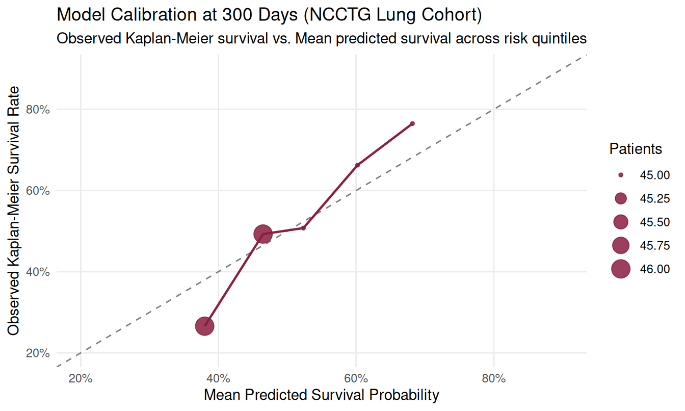

Calibration at 300 days: mean predicted survival versus observed Kaplan-Meier survival within predicted-survival quintiles; the dashed line marks perfect calibration.

Biostatistics Team Entry Point & SAS Macro Suite Guide

This section provides a direct onboarding guide for biostatisticians, statistical programmers, and validation engineers bridging between SAS and R.

Architecture & Workflow Philosophy

TempleCBE is architected with a dual-engine philosophy: - Interactive Development & Visualization: Use R (cox_multi(), explain_survival(), plot_cox_forest()) for agile exploration, nested cross-validation, and publication-ready graphics. - Regulatory Parity & Benchmark Audit: Use SAS (PROC PHREG, %cbe_brier_score, %cbe_cox_phreg) to execute identical models in batch mode and compare the numbers SAS prints with R’s.

Locating Bundled SAS Macros from R

TempleCBE ships with production SAS macros located in inst/sas/. When the package is installed, you can programmatically discover the macro directory or any individual macro file:

# Directory containing all bundled SAS macros
macro_dir <- TempleCBE::sas_macro_dir()
macro_dir
#> [1] "/tmp/RtmppxIjyF/temp_libpath2188179f1d87/TempleCBE/sas"

# Path to the master loader file
master_macro_file <- TempleCBE::sas_macro_path("cbe_macros.sas")
master_macro_file
#> [1] "/tmp/RtmppxIjyF/temp_libpath2188179f1d87/TempleCBE/sas/cbe_macros.sas"

Inside SAS (whether running in SAS Enterprise Guide, SAS Studio, or batch mode), simply include the master loader:

#| lst-label: lst-macro-loader
#| lst-cap: "SAS: Include TempleCBE macro suite via master loader file"
/* In SAS: Include TempleCBE Macro Suite */
%let templecbe_sas = <path_returned_by_cbe_sas_macro_dir>;
%include "&templecbe_sas/cbe_macros.sas";

SAS Macro Catalog & Syntax Reference

The library provides three core macros matching TempleCBE’s R functions:

1. %cbe_brier_score: IPCW Brier Score & IBS Calibration

#| lst-label: lst-macro-brier-syntax
#| lst-cap: "SAS %cbe_brier_score: Macro parameter reference"
%cbe_brier_score(
    data       = <input dataset>,
    time       = <follow-up time var>,
    status     = <event indicator 1/0>,
    pred_vars  = <explanatory variables to auto-fit>,
    eval_times = <space-separated list of milestone times>,
    ties       = BRESLOW,         /* Tie handling: BRESLOW or EFRON */
    trunc      = 0.05,            /* Censoring truncation threshold */
    out_brier  = cbe_brier_scores,/* Time-specific Brier scores */
    out_ibs    = cbe_ibs,         /* Integrated Brier Score */
    out_calib  = cbe_calibration  /* Decile calibration table */
);

2. %cbe_cox_phreg: Standardized Cox Modeling & Assumption Checking

#| lst-label: lst-macro-cox-phreg-syntax
#| lst-cap: "SAS %cbe_cox_phreg: Macro parameter reference"
%cbe_cox_phreg(
    data       = <input dataset>,
    time       = <event time var>,
    status     = <event indicator 1/0>,
    tstart     = <start time var for counting process>,
    vars       = <predictor list>,
    ties       = BRESLOW,
    id         = <cluster/subject ID>,
    assess_ph  = Y,               /* ASSESS PH / RESAMPLE test */
    out_est    = cbe_estimates,   /* Tidy parameter estimates */
    out_fit    = cbe_fit          /* Model fit statistics */
);

3. %cbe_counting_process: Time-Dependent Covariate Reshaping

#| lst-label: lst-macro-counting-process-syntax
#| lst-cap: "SAS %cbe_counting_process: Macro parameter reference"
%cbe_counting_process(
    data_wide  = <wide dataset with P1..Pn>,
    id         = ID,
    time       = Time,
    dead       = Dead,
    obs_times  = 27 34 37 41 43 45 46 47 49 50 51 53 65 67 71,
    var_prefix = P,
    cov_name   = NPap,
    out_data   = cbe_counting_data
);

Running SAS Batch Programs Directly from R (run_sas_script)

TempleCBE provides run_sas_script() to execute SAS batch programs directly from R scripts or test pipelines:

# This code chunk executes automatically when SAS 9.4 is detected on host
sas_benchmark_file <- TempleCBE::sas_macro_path("benchmark_brier_lung.sas")

# Run batch SAS program. By default logs/ and list/ are created beside the script;
# here they go to a temporary folder, so the installed package is not written to.
sas_out <- tempfile("sas_benchmark_")
exit_code <- TempleCBE::run_sas_script(sas_benchmark_file, log_dir = sas_out, list_dir = sas_out)
cat("SAS batch execution completed with exit status:", exit_code, "\n")

run_sas_script() enforces clean separation: - Creates a logs/ directory containing <stem>.log for error/warning auditing. - Creates a list/ directory containing <stem>.lst for formatted ODS outputs. - Returns standard process exit codes (0 = clean execution, 1 = warnings, 2 = errors).

End-to-End Hybrid Workflow: Calling a SAS Macro from R (R $\rightarrow$ SAS $\rightarrow$ R)

In many clinical environments, analysts want to call a validated SAS macro directly on an R data frame without manually writing standalone SAS programs by hand.

The complete round-trip pattern consists of four steps: 1. Export Cohort from R: Write the R dataset to FDA standard transport format (haven::write_xpt()). 2. Compose SAS Macro Driver: Generate a lightweight .sas script invoking the bundled macro (e.g. %cbe_brier_score). 3. Execute via run_sas_script(): Run SAS in batch mode, generating audit logs and listing tables. 4. Import Results into R: Read the generated SAS dataset (haven::read_sas()) back into an R tibble for visualization and verification.

# 1. Prepare R analysis cohort and export to FDA Transport format
lung_xpt_data <- lung_data %>%
  filter(!is.na(ph.karno)) %>%
  rename(ph_karno = ph.karno) %>%
  select(time, status, age, sex, ph_karno)

work_dir <- file.path(tempdir(), "cbe_sas_job")
dir.create(work_dir, recursive = TRUE, showWarnings = FALSE)
xpt_path <- file.path(work_dir, "lung.xpt")
driver_path <- file.path(work_dir, "run_brier_macro.sas")
out_brier_path <- file.path(work_dir, "sas_brier.sas7bdat")
out_ibs_path <- file.path(work_dir, "sas_ibs.sas7bdat")

# Export to standard SAS Version 5 XPORT format (member name <= 8 chars)
haven::write_xpt(lung_xpt_data, xpt_path, version = 5, name = "LUNG")

# 2. Dynamically compose SAS driver invoking %cbe_brier_score
macro_file <- TempleCBE::sas_macro_path("cbe_brier_score.sas")

driver_code <- sprintf('
libname workdir "%s";
libname xfile xport "%s";

/* Copy transport file into SAS WORK library */
proc copy in=xfile out=work;
run;

/* Include TempleCBE macro */
%%include "%s";

/* Execute macro */
%%cbe_brier_score(
    data       = work.lung,
    time       = time,
    status     = status,
    pred_vars  = age sex ph_karno,
    eval_times = 100 200 300 400 500,
    ties       = BRESLOW,
    trunc      = 0.05,
    out_brier  = workdir.sas_brier,
    out_ibs    = workdir.sas_ibs
);
', gsub("\\\\", "/", work_dir), gsub("\\\\", "/", xpt_path), gsub("\\\\", "/", macro_file))

writeLines(driver_code, driver_path)

# 3. Execute SAS batch job from R
status <- TempleCBE::run_sas_script(driver_path)
cat("SAS Macro Execution Status:", status, "\n")

# 4. Import SAS output dataset directly back into R
sas_brier_tbl <- haven::read_sas(out_brier_path)
sas_ibs_tbl <- haven::read_sas(out_ibs_path)

# 5. Display SAS macro results inside R
sas_ibs_tbl
sas_brier_tbl

Calling R from SAS (SAS $\rightarrow$ R)

For statistical programmers working primarily inside SAS Enterprise Guide, SAS Studio, or batch scripts who wish to trigger TempleCBE survival routines or automated Quarto report generation from SAS:

#| lst-label: lst-sas-call-r-systask
#| lst-cap: "SAS SYSTASK: Trigger TempleCBE R script from SAS batch mode"
/* In SAS: Trigger TempleCBE script via OS command */
systask command "powershell -File ""C:\PathTo\TempleCBE\scripts\Rscript.ps1"" -e ""TempleCBE::render_pipeline('vignettes/sas_survival.Rmd', 'all')""" 
    taskname=r_cbe_job wait;

Alternatively, SAS PROC IML supports direct embedded R execution:

#| lst-label: lst-sas-proc-iml-r
#| lst-cap: "SAS PROC IML: Embedded R execution via submit / R block"
/* In SAS: Interactive Matrix Language (IML) R Interface */
proc iml;
    submit / R;
        library(TempleCBE)
        # Execute TempleCBE survival workflows in R
        res <- cox_single(data = survival::lung, outcome = "Surv(time, status)", feature = "age")
        print(res$table)
    endsubmit;
run;

Portable CI/CD Validation Workflow (sas_available())

To ensure scripts, tests, and vignettes run portably across local workstations (with SAS) and CI/CD environments (such as GitHub Actions without SAS), use the conditional evaluation pattern:

# Detect SAS executable on the current host machine:
if (TempleCBE::sas_available()) {
  # Live execution on workstation with SAS
  TempleCBE::run_sas_script("inst/sas/example_85_7.sas")
} else {
  message("SAS not detected on host. Using verified benchmark reference tables.")
}

Beyond Naive Time-Dependent Covariates: Joint Modeling (SAS %JM vs. TempleCBE::joint_model)

Parts 2 and 3 illustrated how time-dependent covariates can be structured into start/stop counting-process intervals via SAS DATA steps or tidy_tmerge_cox(). However, when longitudinal biomarker trajectories are measured with biological noise or subject to informative dropout, treating them as fixed step-functions introduces attenuation bias (Rizopoulos 2010, JSS 35(9); Garcia-Hernandez & Rizopoulos 2018, JSS 84(12)).

To address this: - In SAS: Biostatisticians employ the %JM macro, fitting a joint generalized linear mixed model (PROC NLMIXED with adaptive Gauss-Hermite quadrature) and proportional hazards model. - In TempleCBE: Analysts deploy joint_model() and describe_columns(), which fit coordinated survival (coxnet), binary classification (status), and duration regression (time) models with integrated probability calibration:

# Audit dataset with repeated-measures detection
toy_long <- data.frame(
  patid = rep(1:20, each = 3),
  tstart = rep(c(0, 5, 10), times = 20),
  tstop = rep(c(5, 10, 20), times = 20),
  biomarker = rnorm(60, mean = 50, sd = 10),
  trt = rep(sample(c("A", "B"), 20, replace = TRUE), each = 3),
  status = rep(rbinom(20, 1, 0.5), each = 3)
)
toy_long$surv <- survival::Surv(toy_long$tstart, toy_long$tstop, toy_long$status)

# Audit counting-process duration and baseline vs longitudinal features
audit_res <- describe_columns(toy_long, subject_id = "patid")
audit_res[, c("columns", "class", "variable_type", "mean", "most_freq")]
#> # A tibble: 7 × 5
#>   columns   class     variable_type                mean most_freq               
#>   <chr>     <chr>     <chr>                       <dbl> <chr>                   
#> 1 patid     integer   Subject ID                  10.5  1                       
#> 2 tstart    numeric   Longitudinal (Time-Varying)  5    0                       
#> 3 tstop     numeric   Longitudinal (Time-Varying) 11.7  5                       
#> 4 biomarker numeric   Longitudinal (Time-Varying) 49.4  25.6273638878047        
#> 5 trt       character Baseline (Time-Invariant)   NA    A                       
#> 6 status    integer   Baseline (Time-Invariant)    0.5  0                       
#> 7 surv      Surv      Longitudinal (Time-Varying)  6.67 Counting (Events: 30 [5…

# Fit joint multi-paradigm predictive model
jm_fit <- joint_model(toy_long, surv ~ biomarker + trt, subject_id = "patid", penalty = 0.05)
print(jm_fit)
#> === TempleCBE Joint Survival-Status-Time Model ===
#> Engine: glmnet | Calibration: TRUE
#> Outcome: surv (Type: counting)
#> Sample Size: 60 observations | Predictors: 3
#> Events: 30 (50.0%) | Median Follow-up Time: 10.00
#> Fitted Sub-Models:
#>   1. Cox Survival Model: coxnet_model
#>   2. Status Classification Model: cv.glmnet
#>   3. Time Duration Model: cv.glmnet

SAS to TempleCBE Translation Reference

Task	SAS PROC PHREG Syntax	TempleCBE / R Equivalent
Univariable Screening	model time*status(0) = x / ties=breslow;	cox_single(data, outcome, "x", ties="breslow")
Multivariable Model	model time*status(0) = x1 x2 x3;	cox_multi(data, Surv(time, status) ~ x1 + x2 + x3)
Factor Reference Level	class trt(ref="Control");	relevel_factor(data, "trt", "Control") or factor(trt, levels=...)
Tie Handling	ties=breslow (default) | ties=efron	ties = "breslow" | ties = "efron" (default)
Counting Process (Start/Stop)	model (t1, t2)*status(0) = x;	Surv(t1, t2, status) ~ x
Repeated / Clustered Subjects	id patient_id;	id = patient_id passed via ... in cox_multi()
Time-Dependent Merging	Complex DATA-step macro with arrays/lags	survival::tmerge() or TempleCBE::tidy_tmerge_cox()
Proportional Hazards Test	assess ph / resample;	cox_check(fit) (Schoenfeld tests + interpretation)
Time-Dependent Brier Score	%cbe_brier_score(...)	yardstick::brier_survival(scored, truth, .pred)
Integrated Brier Score (IBS)	%cbe_brier_score(...) -> cbe_ibs	yardstick::brier_survival_integrated(scored, truth, .pred)
Model Calibration Curve	%cbe_brier_score(...) -> cbe_calibration	Quantile grouping + ggplot2
Forest Plot	Custom macro or PROC SGPLOT	plot_cox_forest(res) or plot_cox_forest_multi(res)
Survival Curve vs. KM	baseline out=...; + proc sgplot;	plot_cox_survival(res, overlay_km = TRUE)
Marginal Risk / HR Curve	Custom predict + loess	plot_cox_marginal(res, scale = "hr")
Publication Summary Table	ods output ParameterEstimates=...;	cbe_cox_table(res, sort = "magnitude")
Dataset Pre-Flight Audit	proc contents data=...;	describe_columns(data, subject_id = "...")
Joint Longitudinal-Survival Model	%JM(data=..., survdata=...);	joint_model(data, outcome, engine="glmnet")
Cross-Validated Joint Benchmark	Custom macro loops	cv_joint_model(data, outcome)
Locate Macro Directory	%let dir = ...;	TempleCBE::sas_macro_dir()
Locate Macro File	%include "path/to/macro.sas";	TempleCBE::sas_macro_path("cbe_macros.sas")
Batch Run SAS from R	Command line sas -sysin ...	TempleCBE::run_sas_script("script.sas")

Conclusion

By combining dedicated screening engines, automated assumption validators, flexible argument forwarding, modern time-dependent interval builders, and integrated IPCW Brier score calibration, TempleCBE provides an end-to-end survival modeling ecosystem in R whose PROC PHREG and Brier score results the package tests check against reference values from real SAS runs, while introducing modern tidy programming ergonomics and cross-platform reproducibility for clinical study teams.