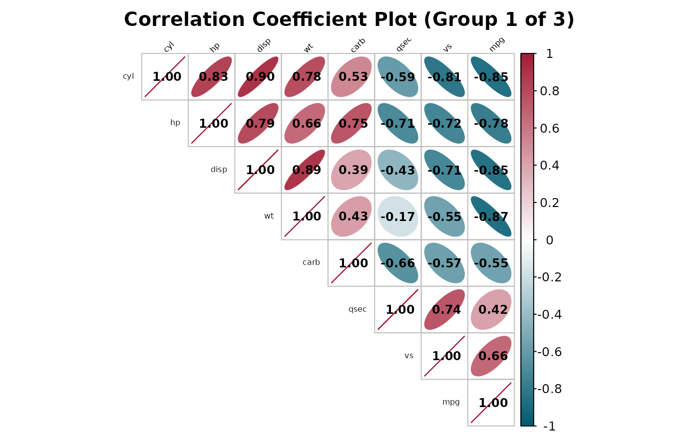
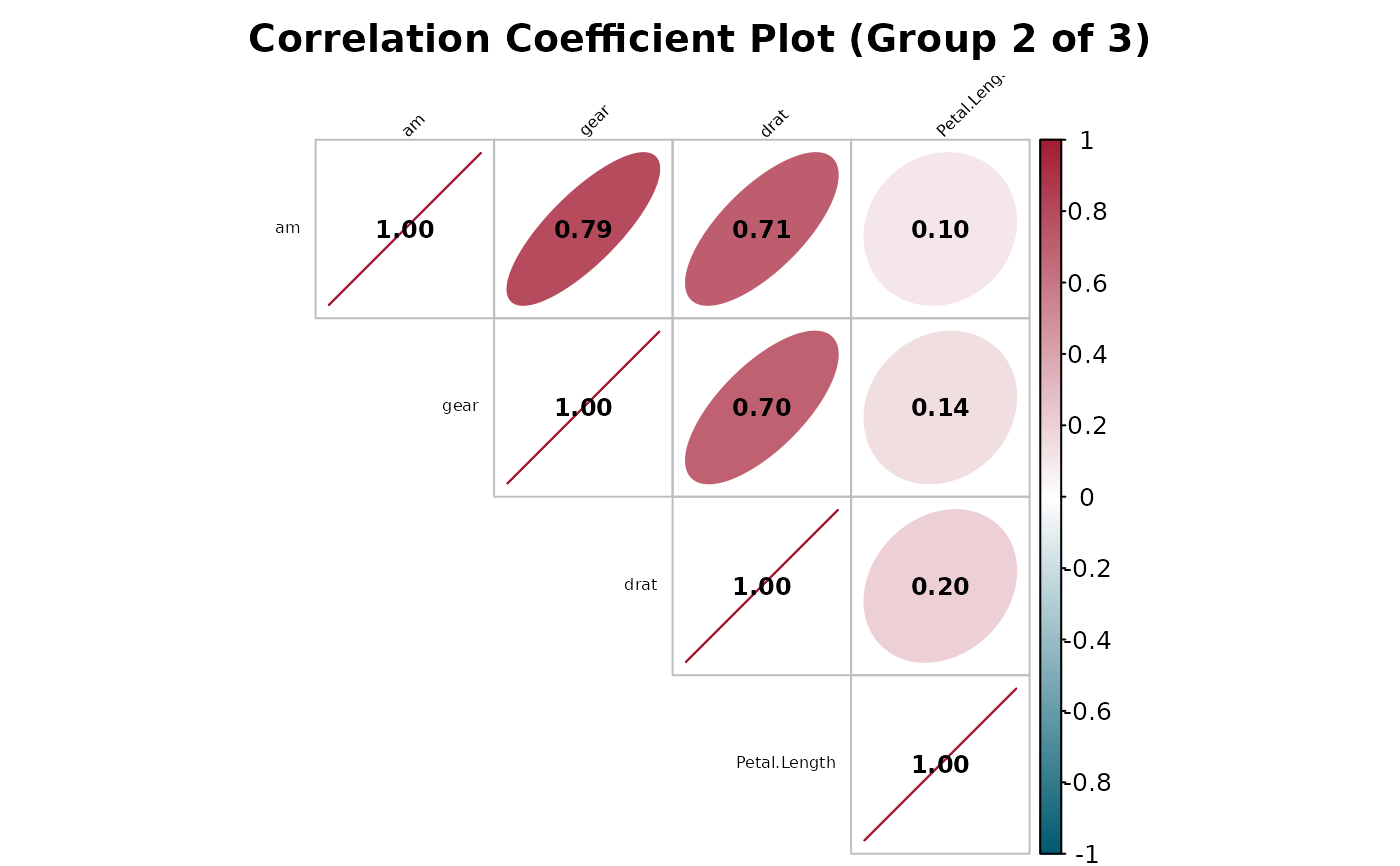
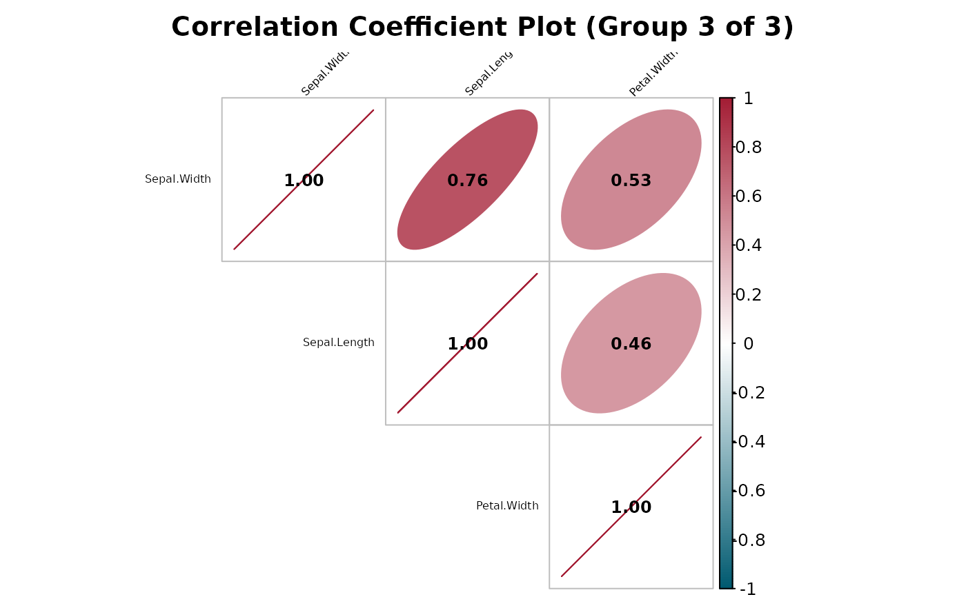
Correlation Plot, Split Into Legible Sub-Plots — correlation_plot

Draws the same style of correlation matrix as correlation_plot, but for matrices with too many variables to stay legible in a single plot (for example, ~40 clinical parameters), it first groups variables via hierarchical clustering on their correlation structure and then draws one correlation_plot-style plot per group, showing only the within-group correlations.

Usage

correlation_plot_split(
  data,
  cor.use = "everything",
  cor.method = "pearson",
  na_omit = TRUE,
  group_size = 12,
  title = "Correlation Coefficient Plot",
  ...
)

Arguments

data: A data frame or tibble.
cor.use, cor.method, na_omit: See correlation_plot.
group_size: Target number of variables per sub-plot (default 12). The number of groups is ceiling(n_vars / group_size); groups may end up somewhat smaller or larger than this target since cutree produces clusters of whatever sizes the dendrogram structure dictates, not exactly equal-sized groups.
title: Base plot title; each sub-plot's title has " (Group i of n)" appended so the sub-plots can be told apart.
...: Additional arguments passed on to correlation_plot for each sub-plot (e.g. tl.cex, show_coef, method).

Value

Invisibly, a named list of per-group correlation matrices (one matrix per sub-plot, named "Group 1", "Group 2", ...).

Details

Variables are clustered on as.dist(1 - abs(cor_mat)) – the same correlation-based distance corrplot's own order = "hclust" uses internally – so that variables which move together end up in the same sub-plot instead of being split arbitrarily (e.g. alphabetically). The resulting dendrogram is cut into ceiling(n_vars / group_size) contiguous groups via cutree.

The default group_size of 12 is chosen to match correlation_plot's own defaults: at the default tl.cex/number.cex, a matrix of roughly a dozen variables is about as many as can fit one legible diagonal label and coefficient per cell without crowding – the same order of magnitude as the small examples (like mtcars's 11 numeric columns) correlation_plot() was originally tuned against. Larger or smaller groups can be requested via group_size depending on label length and plot size.

Examples

# A data frame with more numeric columns than fit legibly in one plot.
wide_data <- cbind(mtcars, iris[seq_len(nrow(mtcars)), sapply(iris, is.numeric)])
correlation_plot_split(wide_data, group_size = 6)