Forest Plot Contrasting the Raw and the Normalized Effect Scale

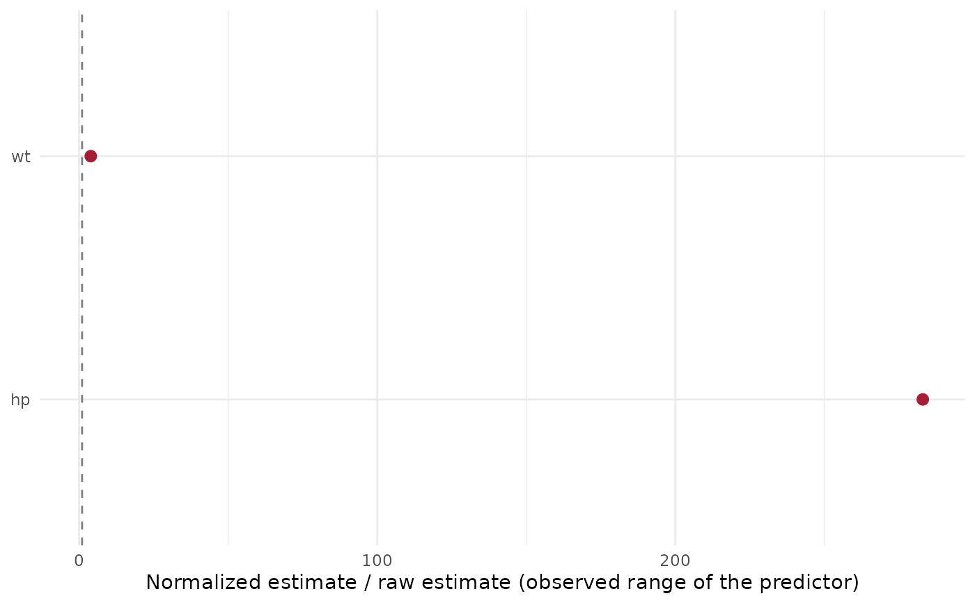
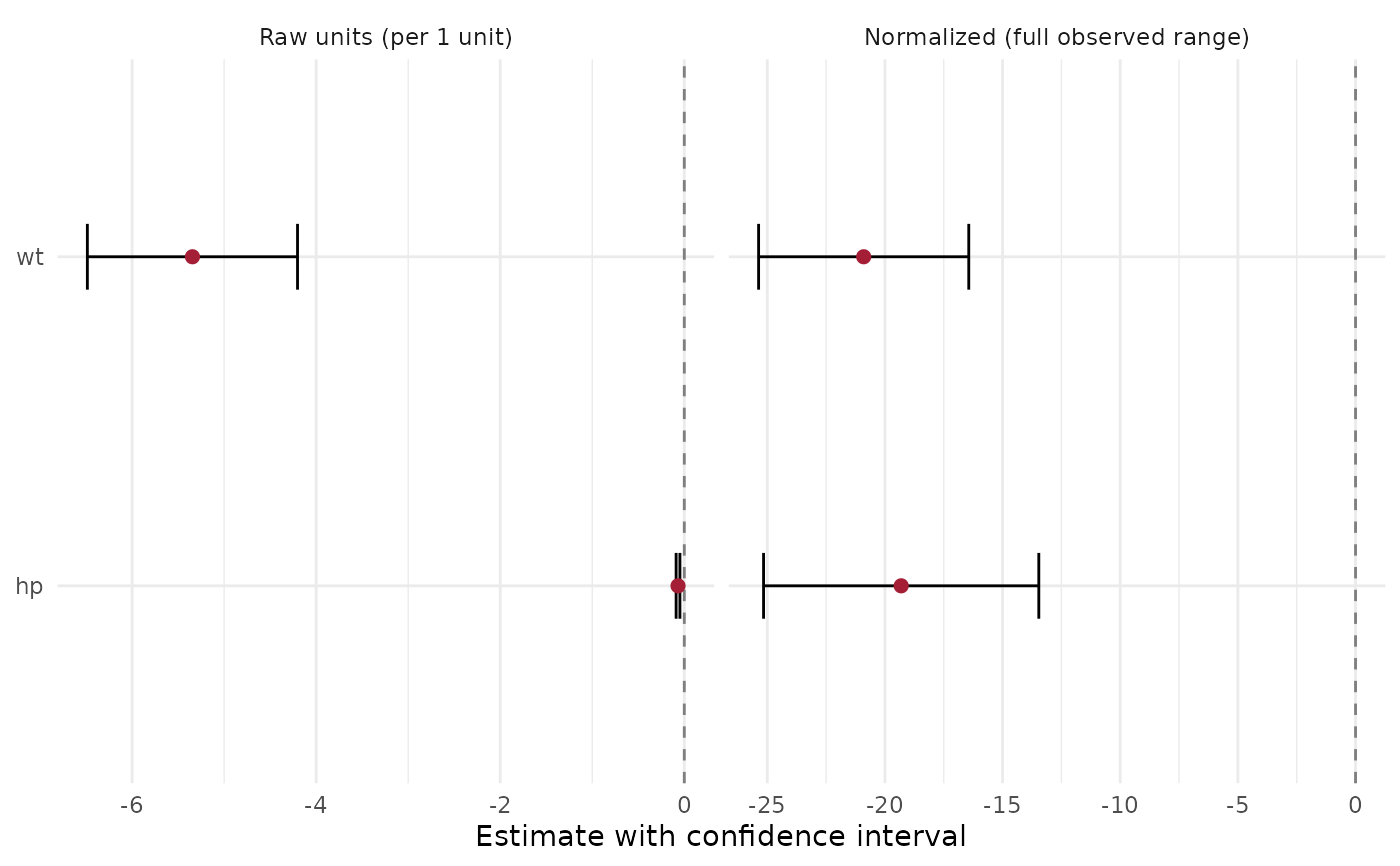
[glm_single()] and [lmm_single()] fit every predictor twice: `scale = "raw"` (change per **one unit**, for example per mm or per kPa) and `scale = "normalized"` (change across the predictor's **whole observed range**). This plot puts the two next to each other, one row per predictor. * `layout = "side_by_side"`: two forest panels with their own axes (raw units on the left, normalized on the right), same row order, so a predictor that looks strong in one scale and weak in the other is easy to spot. * `layout = "ratio"`: one point per predictor, normalized estimate divided by raw estimate. For a linear effect this is the observed range of the predictor in its own unit, which shows how much room each unit-effect has to act. Estimates near zero make the ratio unstable; they are marked when `abs(raw) < ratio_floor`.

Usage

plot_marginal_effect_contrast(
  results_df,
  term_col = "var_label",
  layout = c("side_by_side", "ratio"),
  ratio_floor = 1e-08,
  x_label = NULL
)

Arguments

results_df

Results of [glm_single()] / [lmm_single()] (several can be stacked), with the columns `scale`, `estimate`, `conf.low`, `conf.high`.

term_col

Column that labels the rows (default `"var_label"`).

layout

`"side_by_side"` (default) or `"ratio"`.

ratio_floor

Absolute raw estimate below which a ratio is marked unreliable (default `1e-8`).

x_label

Optional axis label for the side-by-side layout.

Value

A ggplot. Rows whose fit failed (`NA` estimate) are dropped. Its `data` is the wide table (one row per predictor) for `"ratio"` and the long table for `"side_by_side"`.

See also

[plot_coef_forest()], [glm_single()], [lmm_single()]

Examples

res <- rbind(glm_single(mtcars, "mpg", "wt"), glm_single(mtcars, "mpg", "hp"))
plot_marginal_effect_contrast(res)

plot_marginal_effect_contrast(res, layout = "ratio")