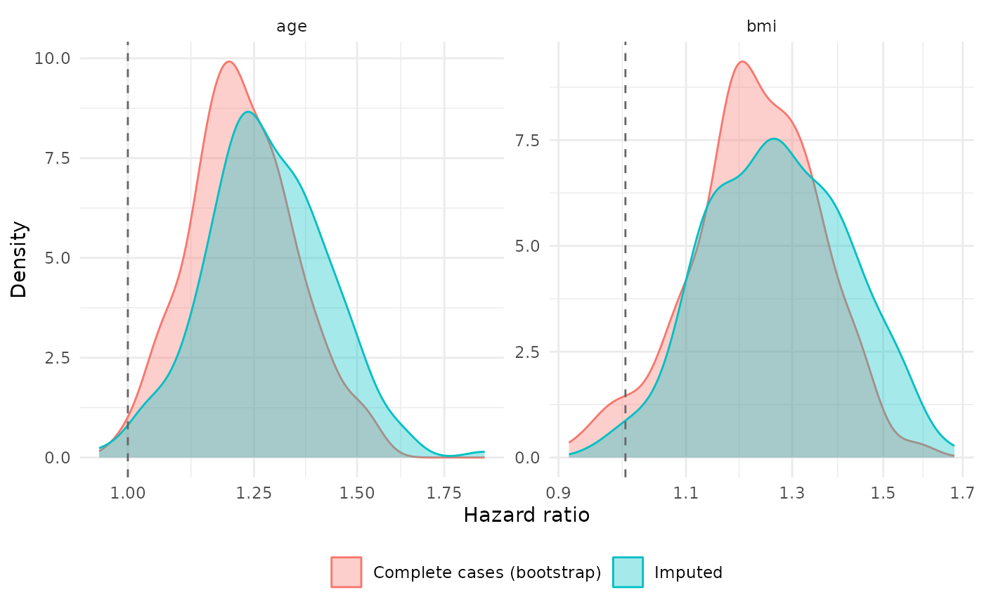
Compare Bootstrap Hazard Ratios Between Complete and Imputed Data

Density overlays, one panel per feature, of the hazard-ratio estimates from Cox models fitted to bootstrap resamples of the complete cases and to imputed datasets. If imputation distorts an effect, the two densities separate.

Usage

plot_imputation_hazard_stability(
  boot_coefs_original,
  imputed_coefs,
  feature_col = "term",
  estimate_col = "estimate",
  exponentiate = TRUE,
  filter_fences = TRUE,
  k = 3
)

Arguments

boot_coefs_original

Data frame of coefficients from the complete-case bootstrap.

imputed_coefs

Data frame of coefficients across the imputed datasets.

feature_col

Name of the feature column in both.

estimate_col

Name of the coefficient column in both (log hazard ratios by default).

exponentiate

Plot `exp(estimate)` (hazard ratios, on a log axis); `FALSE` plots the estimates as they are.

filter_fences

Drop extreme values with Tukey's outer fences (`k` times the IQR beyond the quartiles, computed per feature and source) before plotting. Fitting failures that give huge coefficients otherwise stretch the axis.

k

Fence multiplier: 1.5 for the inner and 3 (default) for the outer fences.

Value

A [ggplot2::ggplot()]. The data after filtering are in `$data`, and the number of removed values per feature and source is in the attribute `n_removed` of the plot.

See also

[km_cutpoints()], [batch_cox_single()]

Examples

set.seed(1)
orig <- data.frame(term = rep(c("age", "bmi"), each = 200), estimate = rnorm(400, 0.2, 0.1))
imp <- data.frame(term = rep(c("age", "bmi"), each = 200), estimate = rnorm(400, 0.25, 0.1))
plot_imputation_hazard_stability(orig, imp)