Visualizations for 2-Way Contingency Tables and Categorical Tests

Generates publication-ready clinical visualizations for 2-way contingency tables with hypothesis test statistics (Central Fisher's Exact Test with mid-p adjustment when zero-cells occur, or Pearson Chi-squared test) automatically formatted in the caption.

Usage

cbe_contingency_plot(
  data,
  var1 = NULL,
  var2 = NULL,
  label1 = NULL,
  label2 = NULL,
  type = c("balloon", "bar", "mosaic", "heatmap", "square", "corrplot"),
  bar_position = c("fill", "dodge", "stack"),
  engine = c("ggplot", "corrplot", "ggpubr"),
  test = c("auto", "exact", "chisq", "fisher"),
  correct = FALSE,
  size_range = c(6, 22),
  fill_colors = c("#F4F4F4", "#9D2235"),
  show_counts = TRUE,
  title = NULL,
  caption = NULL,
  p_format = NULL,
  ...
)

contingency_plot(
  data,
  var1 = NULL,
  var2 = NULL,
  label1 = NULL,
  label2 = NULL,
  type = c("balloon", "bar", "mosaic", "heatmap", "square", "corrplot"),
  bar_position = c("fill", "dodge", "stack"),
  engine = c("ggplot", "corrplot", "ggpubr"),
  test = c("auto", "exact", "chisq", "fisher"),
  correct = FALSE,
  size_range = c(6, 22),
  fill_colors = c("#F4F4F4", "#9D2235"),
  show_counts = TRUE,
  title = NULL,
  caption = NULL,
  p_format = NULL,
  ...
)

balloon_plot(
  data,
  var1 = NULL,
  var2 = NULL,
  label1 = NULL,
  label2 = NULL,
  engine = c("ggplot", "corrplot", "ggpubr"),
  size_range = c(6, 22),
  fill_colors = c("#F4F4F4", "#9D2235"),
  show_counts = TRUE,
  title = NULL,
  ...
)

bar_plot(
  data,
  var1 = NULL,
  var2 = NULL,
  label1 = NULL,
  label2 = NULL,
  bar_position = c("fill", "dodge", "stack"),
  show_counts = TRUE,
  title = NULL,
  ...
)

mosaic_plot(
  data,
  var1 = NULL,
  var2 = NULL,
  label1 = NULL,
  label2 = NULL,
  show_counts = TRUE,
  title = NULL,
  ...
)

heatmap_plot(
  data,
  var1 = NULL,
  var2 = NULL,
  label1 = NULL,
  label2 = NULL,
  fill_colors = c("#F4F4F4", "#9D2235"),
  show_counts = TRUE,
  title = NULL,
  ...
)

four_quadrant_report(
  data,
  var1 = NULL,
  var2 = NULL,
  label1 = NULL,
  label2 = NULL,
  test = c("auto", "exact", "chisq", "fisher"),
  correct = FALSE,
  p_format = NULL,
  ...
)

square_plot(
  data,
  var1 = NULL,
  var2 = NULL,
  label1 = NULL,
  label2 = NULL,
  test = c("auto", "exact", "chisq", "fisher"),
  correct = FALSE,
  engine = c("ggplot", "corrplot"),
  size_range = c(6, 22),
  fill_colors = c("#F4F4F4", "#9D2235"),
  show_counts = TRUE,
  title = NULL,
  caption = NULL,
  p_format = NULL,
  ...
)

Arguments

data: A data frame containing the categorical variables, or a 2-way table/matrix.
var1: Character string of the row variable column name (ignored if data is a table).
var2: Character string of the column variable column name (ignored if data is a table).
label1: Optional display label for var1 (defaults to var1).
label2: Optional display label for var2 (defaults to var2).
type: Visualization type: "balloon" (default), "bar", "mosaic", "heatmap", "square", or "corrplot".
bar_position: Position adjustment when type = "bar": "fill" (100% proportional stacked bar, default), "dodge" (side-by-side grouped), or "stack" (count stacked).
engine: Engine for balloon/square rendering: "ggplot" (default), "corrplot", or "ggpubr".
test: Hypothesis test engine: "auto" (default CBE hierarchy), "exact" (force Central Fisher exact test for 2x2 or simulated Fisher for RxC), "chisq" (force Pearson's Chi-squared test via chisq.test), or "fisher" (force fisher.test).
correct: Logical; whether to apply continuity correction when test = "chisq" (default FALSE following CBE standard protocol).
size_range: Numeric vector of length 2 giving min and max glyph sizes for balloon and square plots (default c(6, 22)).
fill_colors: Character vector of colors for the palette or gradient. Defaults to Temple University brand palette (c("#F4F4F4", "#9D2235")).
show_counts: Logical (default TRUE); whether to print cell counts inside plots.
title: Plot title. If NULL, defaults to "{label1} \u00d7 {label2}".
caption: Optional plot caption. If NULL, automatically computed and formatted using pformat with test description.
p_format: Optional p-value formatting function (default pformat).
...: Additional arguments passed to underlying plotting functions.

Value

A ggplot object (for "balloon", "bar", "mosaic", "heatmap", "square"), or invisibly the contingency table (for "corrplot").

Details

Supported visualization types:

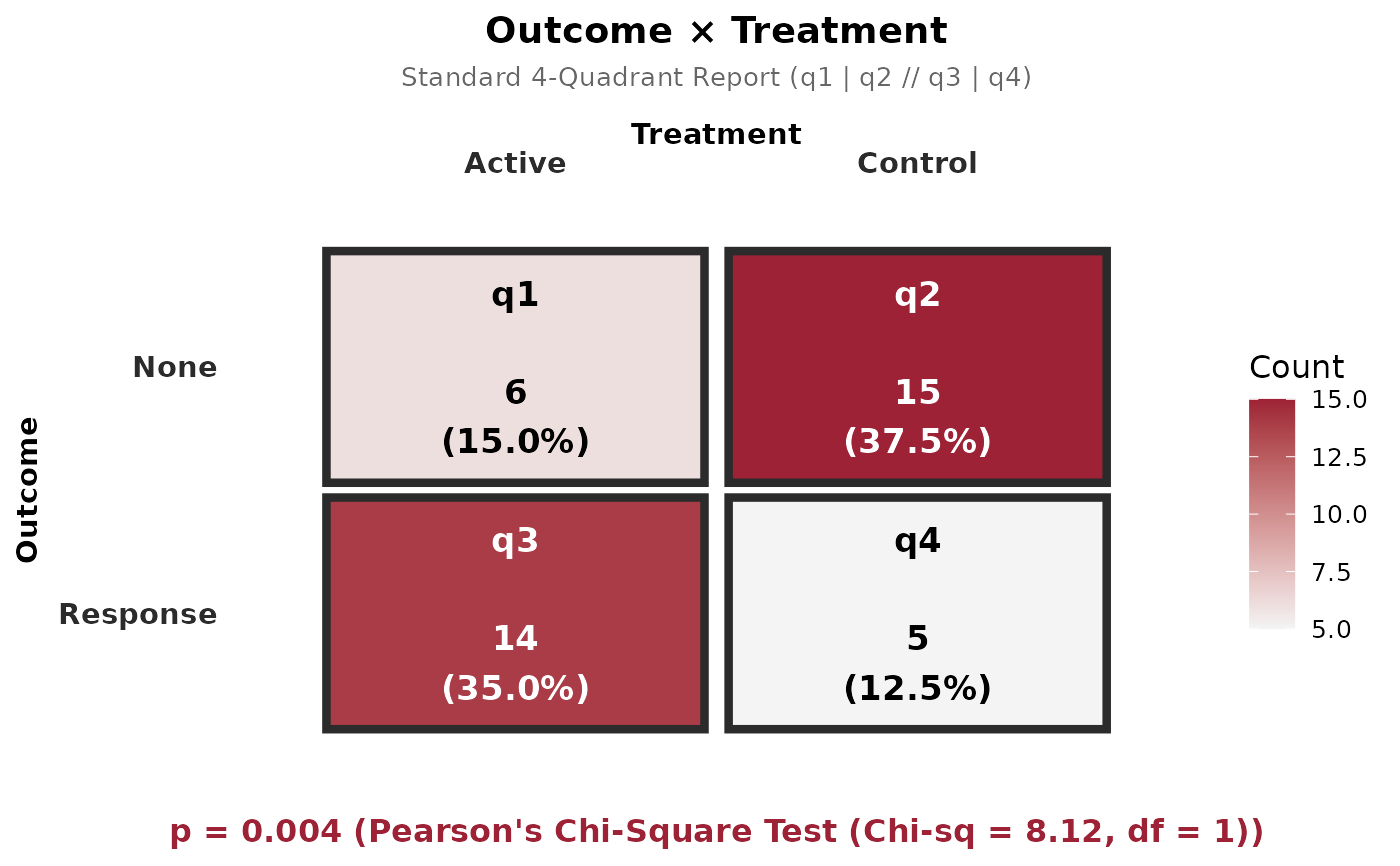
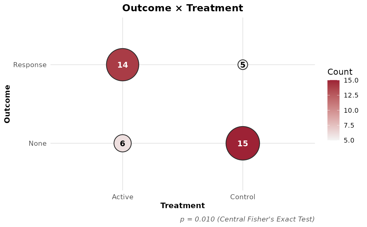
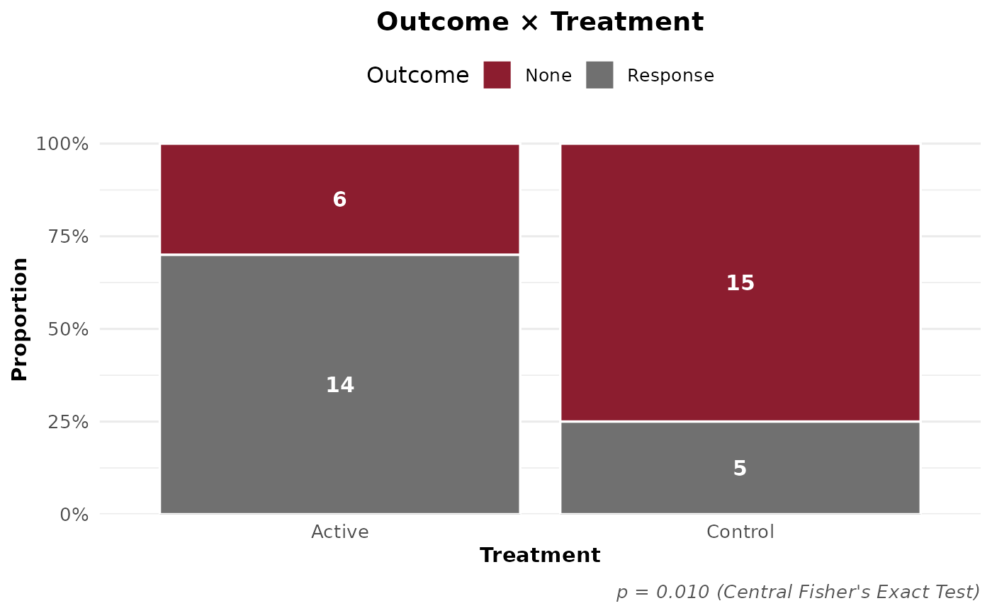
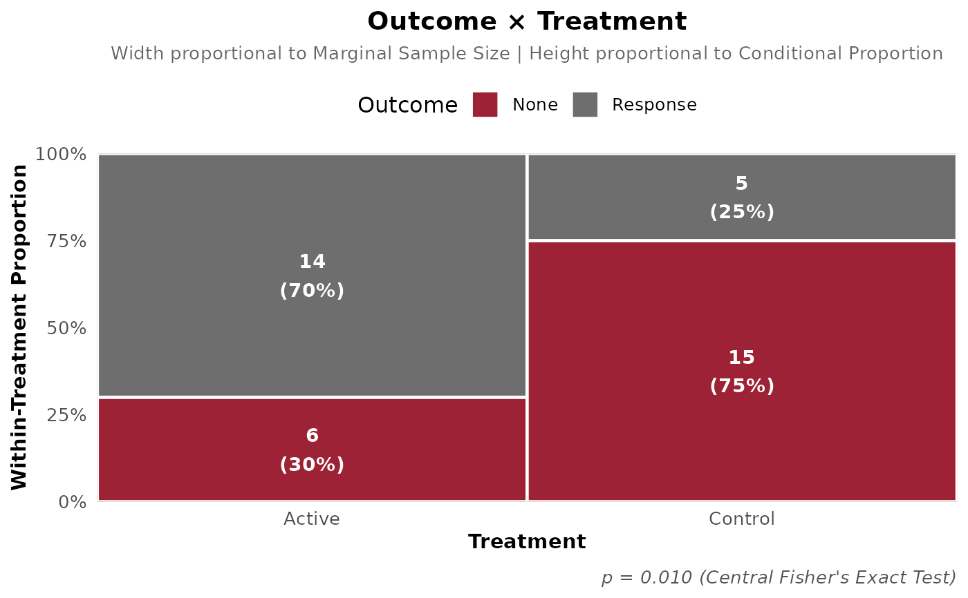
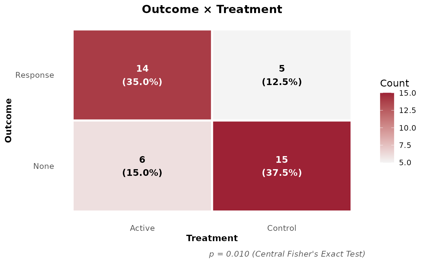
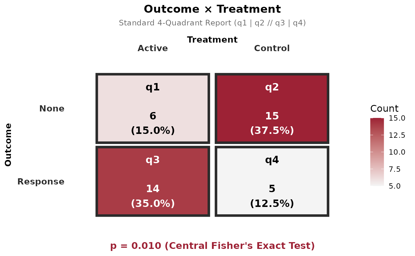
"balloon" (default): Proportional bubble/circle plot with counts displayed inside circles.
"bar": Grouped, stacked, or 100% proportional fill bar chart.
"mosaic": Two-dimensional mosaic plot with tile area proportional to joint frequency.
"heatmap": Shaded tile heatmap with cell frequencies and overall percentages.
"square": Standard 4-quadrant report for 2x2 tables (q1 | q2 // q3 | q4 // p = pformat), or proportional square tiles for RxC tables.
"corrplot": Circular or square matrix plot rendered via corrplot.

Examples

df <- data.frame(
  Treatment = factor(c(rep("Active", 20), rep("Control", 20))),
  Outcome   = factor(c(rep("Response", 14), rep("None", 6),
                        rep("Response", 5), rep("None", 15)))
)

# 1. Balloon Plot (Temple Brand Colors)
cbe_contingency_plot(df, "Outcome", "Treatment", type = "balloon")


# 2. Proportional Bar Plot (100% Fill)
cbe_contingency_plot(df, "Outcome", "Treatment", type = "bar", bar_position = "fill")


# 3. Mosaic Plot
cbe_contingency_plot(df, "Outcome", "Treatment", type = "mosaic")


# 4. Heatmap
cbe_contingency_plot(df, "Outcome", "Treatment", type = "heatmap")


# 5. Standard 4-Quadrant Square Plot (q1 | q2 // q3 | q4 // p = pformat)
cbe_contingency_plot(df, "Outcome", "Treatment", type = "square")


# 6. Force Pearson Chi-Square Test
cbe_contingency_plot(df, "Outcome", "Treatment", type = "square", test = "chisq")